Harrod Domar Model
What HD model does?
Its purpose is to identify the necessary condition for achieving steady economic growth. It is a post-Keynesian Model, developed in 1930 – 1940s.
Formula:
g = s / θ – δ (No population growth)
- where g is the output growth rate
- s is the saving rate
- θ is the capital / output ratio
- δ is a fraction of capitals that depreciate
g = s / θ – δ – n (With population growth)
- n is the population growth
Assumptions:
- Fixed savings rate and capital output ratio
- constant return to scale
- No technological progress
Dynamics:
To encourge higher growth, policy makers should:
- Encourage higher saving and investment (increase s)
- Increasing labour productivity (Lower the capital output ratio)
- Increasing capital efficiency (Lower depreciation rate)
- reduce population growth (lower n, as growth is on per capita basis)
Prediction:
- No Convergence on growth: conditional on the same set of parameters, all countries will growth at the same rate, if starting at different level of parameters, there will never be catch-up in growth because of constant return to capital.
Critique:
- Although increase in investment lead to increase in economic growth, it does not explain growth by sectoral compositions; such as whether the growth is from rural or urban sector investment is unknown.
- All inputs are exogenous, saving rate, capital output ratio, population growth, all independent from per capita income levels. In reality, these factors are endogenous to growth, and have a more complex dynamics. E.g.: In short-term, low population growth with increased growth rate; In the longer time frame, increase in income lead to higher population growth rate. It is therefore hard to increase its per capita income.
Solow Model
What Solow model does?
Its purpose is explaining long-term economics growth. It addresses many flaws of HD Model.
Formula:
It is derived from Cobb-Douglas production function:
- Y = AKa L1-a, where A is the Technical Progress factor; K is the capital, L is the labour, a is the capital share of output.
- If a = 1, then it would be HD model, where it is constant return to scale.
- Instead Solow Model assume a < 1, where it is decreasing return to scale
- Most developed countries have a = 1/3
Solow Model Capital Dynamics:
- Capital in the economy can be represented by net old capital (after removing depreciation) plus the new investment (a fixed saving ratio * output)
- K(t+1) = (1 – δ)Kt + sYt
- Now, capital per capita taking into the popultaion growth rate (n) can be represented as:
- k(t+1) = [(1 – δ)kt + syt]/(1 + n)
Assumptions:
- Based on Cobb-Douglas with K, L as input.
- K has decreasing return to scale, meaning per capita growth will grow at a decreasing speed over time.
- Take into acount of population growth rate (n), as a discount factor
- With Technological Progress will affect the long-run steady state at a growth rate of π.
Prediction 1: (WIthout Technical Progress)
- There is a Conditional Convergence
- Long-run growth rate gradually slows down to 0.
- Short-run growth rate can be raised or lowered by changing s, n, δ.
- Conditioning on the same set of parameters poorer countries can achieve faster growth rate. Difference in per capital income will tend to narrow down over time due to diminishing return on capital.
- Converge on the same set of parameters.
- If parameters are not the same, then there is no convergence.
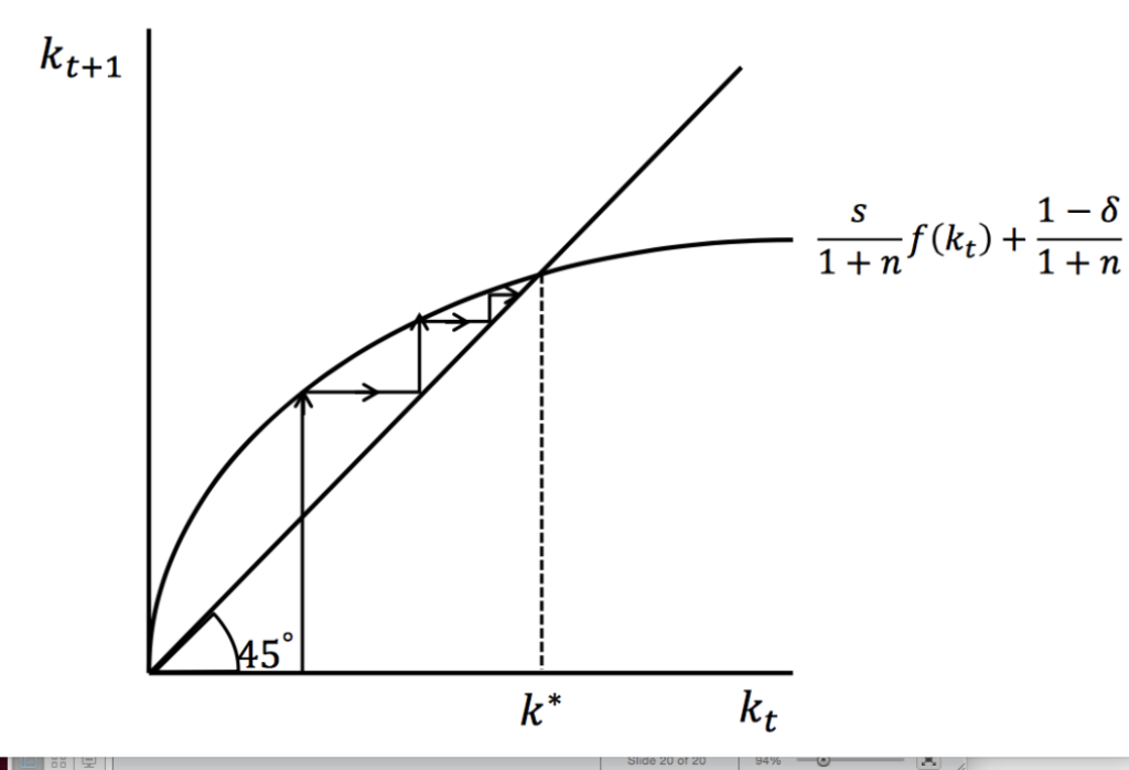
Prediction 2: (With Technical Progress)
- Technical progress can, to some degree, offset the impact of diminishing return on capital.
- The technical progress increase the effective labour (AL), meaning more productive labour
- The small k, is initially calculated as big K divided by L, meaning the capital per labour; now taking into account technical progress A, now become capital per effective labour(K/AL). As a result, k = K/AL, and the value is decreased.
- When k get smaller, the impact of dimishing return is delayed, enable the per capita income to kept on increasing.
- There is conditional convergence
- Long-run growth rate is equal to its Technological Progress Rate (π, assumes π > 0)
- Short-run growth rate depends on the value of parameters (s, n, δ).
- Convergence one the same set of parameter.
- If parameter are not the same, there is convergence on growth rate at π, but no convergence on income per capita.
Evidence of conditional convergence:
- Southeast Asia countries enjoy higher growth than western countries in the period of 1960-1980s. They are not starting with same set of parameters. As developed economies usually have higher level of saving, lower level of depreciation and population growth, they are at a higher level of capital curve. However, western counrties experience diminishing return on capital as capital stock accumulates. On the other hand, southeast starting with lower of level of capital stock, and therefore there is less penality on diminishing return on capital.
Evidence of non-convergence:
- We also observe divergence across region, developed countries kept a steady rate of growth, while the poorer countries did not experience a significant catch-up effect.
- For instance, Latin America and Sub-Saharan Africa, whose rate of return on capital has been low steadily.
Limitations: We assume all countries have the same rate of technological progress rate, due to free flow of knowledge. Hence, we also assume that all new technology is immediately available everywhere and that capital costs are not assumed. Paul Romer think there is ‘Black Box’ for tech development, lacking free flow of tech.
Lewis Model
What Lewis model does?
It explains why labour surplus is a driver of industrial growth.
Assumptions:
- Dual-Sector Economy: Agriculture & Manufaturing
- Two resources flow help the economic development (food & labour)
- There is surplus of labour in agriculture, removing them from land have no impact on output, therefore the marginal product = 0
- Capital intensive industrial sector has higher productivity than agriculture sector.
- Organisation of production: Sharing family income in agriculture vs paying market wages (MPIL) for hiring in the industrial sector.
- Closed Economy, no food import.
Predictions:
- Development Pattern is not even;
- Benefit of develpment in the early stage accrue entirely to capitalists
- Inequality rises in the early stages, benefits flow down to workers only in the last stage.
Three Stages Dynamics:
- First Stage:
- Output is constant in agriculture (Marginal Product is zero)
- Labour can flow to modern sector, without penality on food production
- Second Stage:
- Disguised Unemployement: It cost more too feed a worker than his contribution to the output in the agriculture.
- 0 < MPaL < APaL = Wa
- Marginal product increases above 0. This pushes the average product of agriculture higher, as a result, the wage is higher for agriculture worker (equal to average product in agriculture).
- Average surplus of food goes down as agriculture output decrease, leaving less food for the worker in the industrial sector. It drives up food price, and pushes the industrial wages higher. Therefore, lower profit for the industrial sector.
- Third stage:
- Each worker contributes more than he is getting paid in agriculture.
- MPaL > Wa
- Wages will increase for agriculture, and less surplus labour for the industry.
- Transfering labour from agriculture to industrial sector is no longer possible due to labour scarcity.
- Commercialisation of agriculture.
Graphical Illustration of Three Stages:
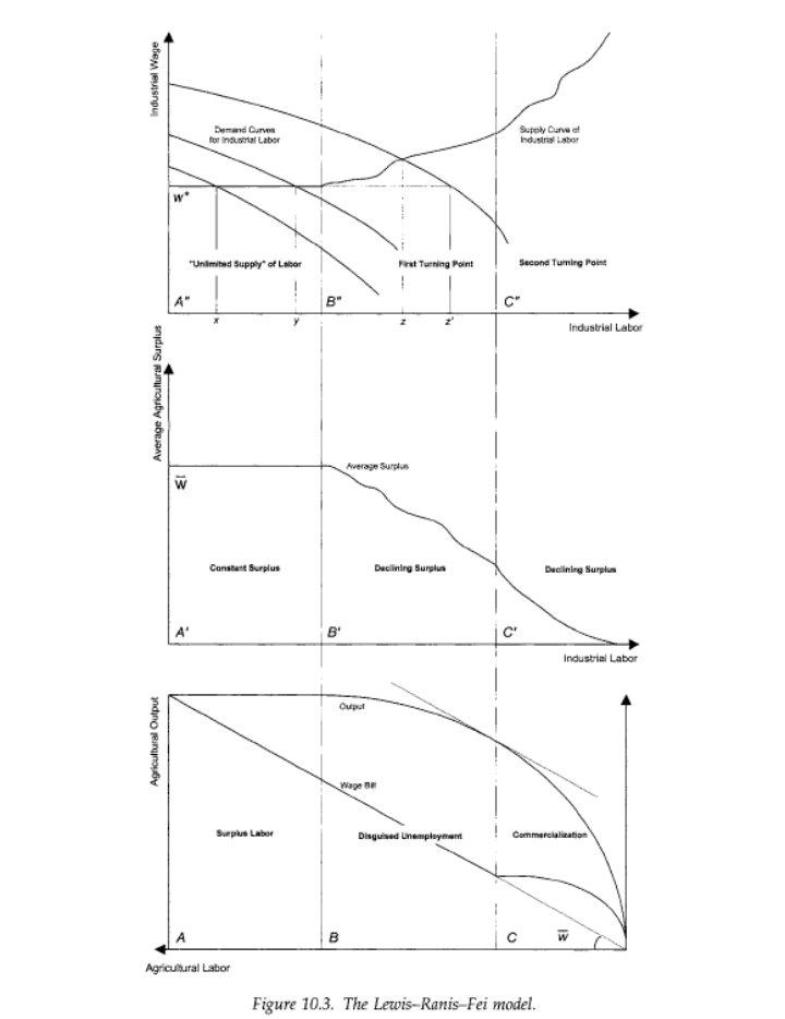
- First diagram shows how industrial wages go up from second stages onwards due to rising food price, and less surplus of agricultural workers.
- Second diagram shows a decreasing agriculture surplus from second stage, as the cost of feeding a labour is greater than his output. Transfering of surplus labour become increasing difficult entering to the third stage, as less and less agricultural surplus labour is available
- Third diagram shows a decrease agricultural output, as marginal product of agricultral labour > 0 entering into second stage where transfering of surplus of labour has substantive impact on the agriculture output. It enters into disguised unemployment (0 < MPaL < APaL = Wa), and later in the third stage enters into agricultural commercialisation (MPaL > Wa).
Critques:
- Once an industrial sector and capitalist class emerges, development proceeds automatically (similar to Solow growth process)
- Rate of growth decrease due to lacks of surplus labour and food, unlike Solow model which is due to diminish return to capital
Harris Todaro Model
What HT model does?
It explains why rural individuals migrate to urban area despite high umemployment in Urban Area.
Assumptions:
- No unemployment in rural areas, flexible labor markets with no minimum wage regulation (WA = MPRL).
- No surplus of Labour, there is no first stage like the Lewis model where the agriculture output unchanged with loss of agriculture labour.
- Urban formal sector (minimum) wage is set at a level that exceeds rural wage (WM > WA).
Dynamics:
- Rural workers are attracted to modern sector where they can get a formal job that pays a higher wage.
- Earning in urban informal urban sector are zero
- There is a probability (p) that a rural migrant does not get a formal job.
- LU = L – LA
- LM =LU – LI (LI means labour in urban informal sector)
- Migration happens only when: (p * WM) > WA
- Also, (LM / LU) = (WA / WM), the share of labour in the manufaturing sector as a proportion of urban workforce equal to the ratio of agricultural wage to the formal urban wage.
Graphical Illustration:
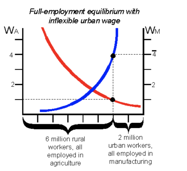
The inflexibility of Urban wages refers to wages in the urban formal sector does not adjust downwards even with a presence of high umemployment. Therefore, only rural wage will adjust as you will see in the last graph of final equilibrium.
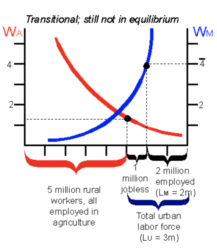
When 1 million worker flow from rural to urban, instead of getting employed in formal sector, they all goes jobless in the informal sector.
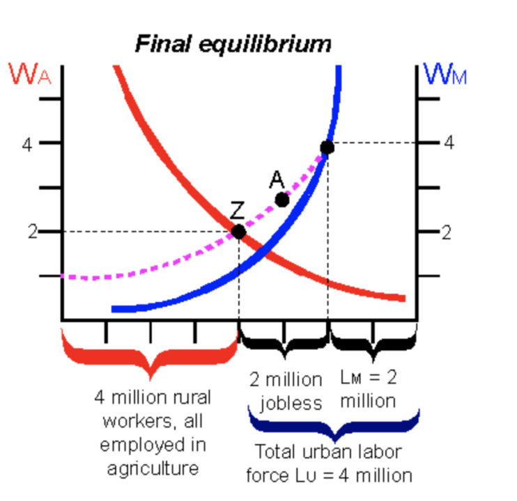
As more and more rural labor flows to urban area, the labour supply in the rural sector shrinks. With fewer rural workers, the marginal product to capital increases in rural area as fewer labour sharing the same amount of land and resources. As WA = MPRL, the wages in rural sector increases, and reflected as an upward movement in Labour demand curve. The final equilibrium is at Z.
Lorenz Curve
What Lorenz Curve does?
It illustrates the income or wealth distribution of a population.
Formula:
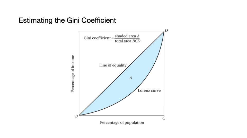
- The greater the curvature of the Lorenz curve, the greater the relative inequality.
- Gini Coefficient: The ratio of the shaded area under the line of equality dividided by the total lower triangle area. Notice the y axis is percentage of income and x axis is the percentage of population.
- Gini = 1 means perfect inequality

- All pairwise comparison are normalised based on the number of pairs and the mean.
Dynamics:
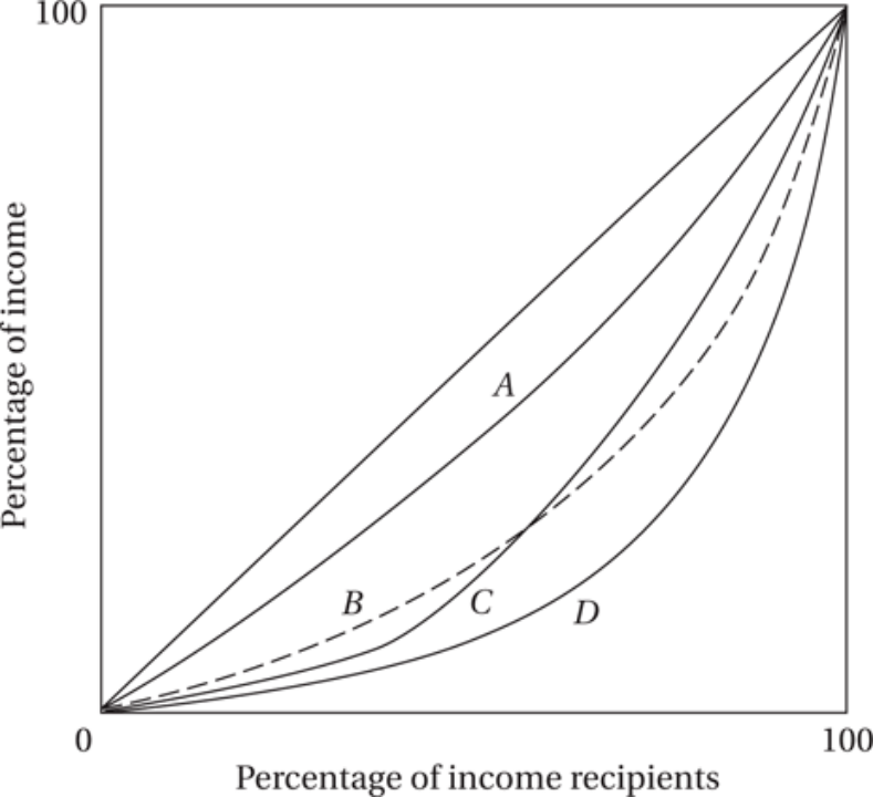
- Lorenz curve can cross! Therefore, we can not say inequality is higher in one case than the other.
- In this case, B has bigger inequality in the upper income class than C.
Applications:
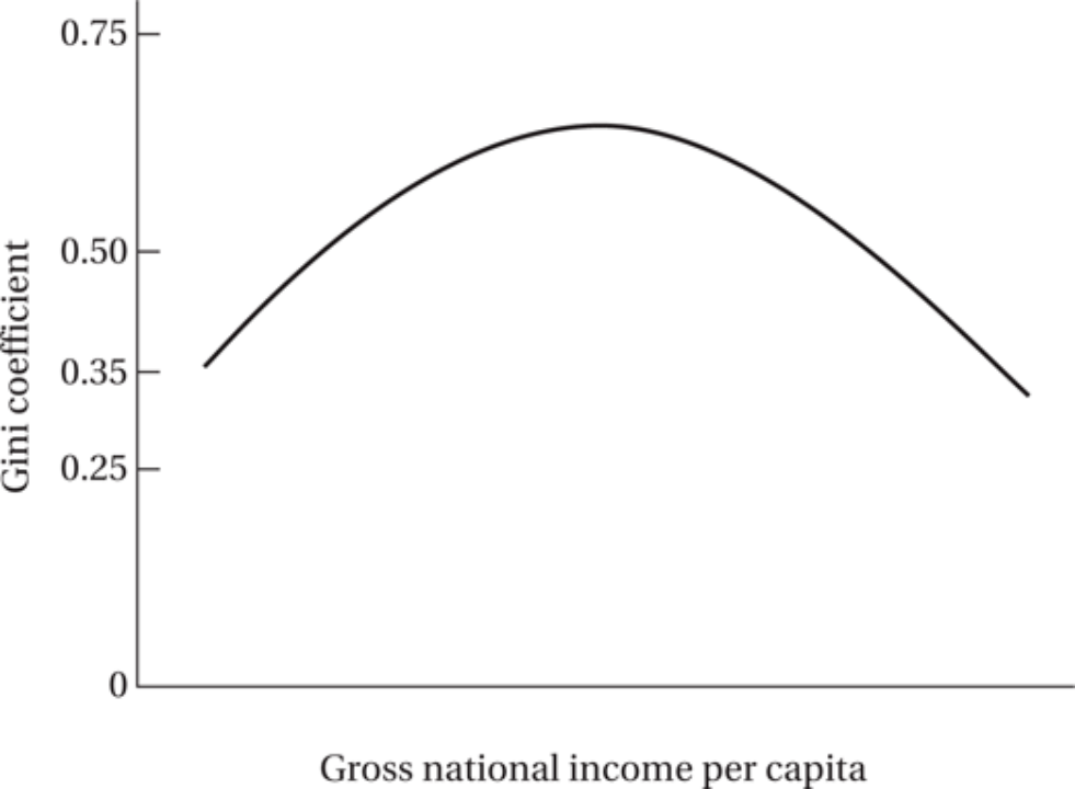
Kuznet Curve:
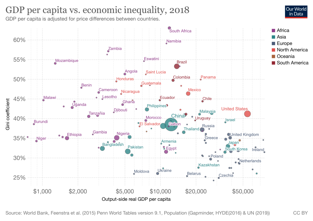
- Kuznet shows the relationship between growth and inequality
- Similar to Harris Todaro model, it also examine the impact of rural migration. As workers moves form agriculture to industry, there is higher inequality as industrial sector has higher mean income and when industry is small, there is an increase in inequality.
- Over time, as industrial sector gets bigger, the demand for unskilled labour increases and inequality decreases.
- Uneven growth: Inequality rises up at the start, because industrialisation and technical progress may be labour saving. Therefore, it is biased against unskilled labour and creating unemployment
- Compensatory growth: over time, inequality is reduced, demand is generated for unskilled labour via service, wage increase
Some Questions with Solutions, (6SSPP333)
Section A (12 mins per question)
Ques 1: In the Lewis Dual economy model, the phrase of disguised unemployment must be associated with a horizontal supply curve of labour. Is this CORRECT? (13 marks)
Ans: False
disguised employment usually happens at the second stage of Lewis dual economy model, where the cost of feeding a agricultural worker is higher than its contribution to the output in the agriculture economy.
The disguised unemployment happens when the availability of surplus on agricultural labour decreases. As a result, the marginal product of agricultural labour is bigger than 0, the loss of agricultural labour will reduce the output on food. The supply of food per capita goes down, the food price goes up relative to industrial goods. This drives up the living cost of industrial workers, therefore the norminal wages for industrial workers goes up which lead to a upward sloping supply curve for industrial workers.
Ques 2: In the Lewis Model, the supply curve of labour to industry is steeper when the economy is closed to subsistence level to begin with. Is this CORRECT?
Ans: False
If a economy is close to subsistence level, the first stage of the Lewis model will be very short, as the peasants want to eat more instead of keeping their initial consumption level, and let industrial workers enjoy stable food prices.

Lewis Model assumes that agricultural workers will not increase their consumption, when the average product of agricultural workers increases. At the first stage of the Lewis Model, the marginal product of agricultural product = 0. The agriculture output can maintain its level even with flowing out of the agriculture workers. The same share of agricultural output will be availble for purchase by the workers who re-allocated to the manufacturing sector. There is no increase in food price, and therefore, the norminal and real wage remain the same.
When economy transition to the second stage, there is less surplus of agricultural worker available. Therefore, the food price goes up, as the marginal product > 0. This pushes up the cost of living for industrial worker, which results in norminal industrial wages. At the second stage, the supply curve is upward sloping, but not too steep, as there is still surplus labour available.
However, subsistence level meaning that people in agricultural sector are near starving. Hence, the assumption on not increasing consumption when higher average surplus available will not hold. Therefore, there are less food remaining for industrial workers. The transition from stage 1 to stage 2 will be faster than Lewis Model with original assumption. The second stage norminal wage in manufaturing need to rise faster than the increasing food price to offset the acute food shortage problem and fast rise of fodd prices.
The amount of food available for industrial workers declines in the second stage because:
- Total agricultural output falls
- peasant eat too much
Therefore, the slope of the second-stage supply curve goes a lot steeper.
Ques 3: In the Lewis Model, the supply curve of labour to industry is flatter when food can be freely traded on the world market. Is this CORRECT?
Ans: True
Although the original Lewis Model assumes a closed economy, where there is no import or export of food. We can conceive what would happen if this assumption is relaxed.
If we assume that our country can freely import food from abroad. Domestic food prices will be lower compared to the sitution with no food import allowed, and the industrial wage rate can be kept at a relatively lower level. As a result, the domestic agricultural sector plays a less import role in providing food to industrial sector. Thus, there will be more surplus of agricultural labour. The cost of feeding an agricultural worker is not higher than the average output they produced, due to cheaper food import. It prolongs the period of rapid industrial growth in the first and second stages. With cheaper food price, real industrial wages can increase without needing greater increase in norminal wages, making the supply curve of industrial worker flatter.
Evidence: The Corn Law in Britain from 1816 to 1845, there were a series of import tariff imposed on grain; which raised the food prices and indirectly related to the Irish Potato Farmine. Higher food price raised the subsitence wage of industrial workers and encourages the agriculture worker to consume the food that they produced. This drives up the wages in the industrial sector and creating a steeper supply curve, thus, it reduces the profitability of industrial expansion. Result: By limiting the availability of cheap food, the Corn Laws indirectly hindered Britain’s Industrial growth during their enforcement
Ques 4:If we know the depreciation rate, the population growth rate and the savings rate, and the capital output ratio we can compute the growth rate of a country. True or Not?
Ans: True
We can either use Harrod Domar. Which both utilised these parameters.
The growth rate can be obtained using Harrod Domar model: growth rate = saving rate / capital output ratio – depreciation rate – population growth. Where the higher the saving rate the higher the growth rate as more investment injected into the economy. Lower capital output ratio lead to higher growth because there are higher labour productivity. Lower depreciation lead to high growth due to more retained capital and capital efficiency. Reduction on population growth can boost the economic growth on a per capita basis.
The HD model assuem a fixed saving rate and capital output ratio and constant return to scale. It is sufficient to calculate the growth rate as it does not require addition parameter such as technical progress factor. All parameters are exogenous to the growth rate.
For Solow Model, we need technical progress.
Ques 5: In the Solow model, labour saving technological progress pushes the production frontier out but by smaller and smaller amounts, due to diminishing returns to technology.
Ans: False
The rate of technical progress is a constant value and not suffer from diminishing return. It is the long-term growth rate for all economies.
Effective units of Labour reduce the value in the denominator for Xt, capital per effective labour. Therefore, xt < kt; therefore delay the condition convergence at a steady state. It shift the capital dynamic curve upwards.
Ques 6: Higher inequality causes lower growth.
Higher inequality correlated with lower growth, not neccessarily causation.
It permits one individual cetain material choices, denying other people for the same choice.
Higher inequality Lower growth:
Inverted U shape Kuznet curve, developed in 1950s by Simon Kuznets.
- inequality increase until a tipping point.
- short run lower growth
- in the long run, inequality does not cause lower growth.
- Gini index 0 is good
Easterly (2007): good vs bad inequlity
- Bad: inequality emerges with historical events
- ‘Elite’ created from slavery and land distribution
- Inequality led to lower levels of per capita income
- Good: Inequality from market movement
- eventually, it will lead to structual development and growth
HIgher inequality higher growth
classsical approch:
- Marginal propensity to save increase with income
- Inequality lead to greater saving via hyper-rich.
- People will save more with income increase
- Redistribution policy will then reduce this growth
- ### Not really ‘Moral‘
Galor and Zeira Model:
- Theoretical linkage between income distribution and macroeconomics through investment in human capital.
- credit market are imperfect due to imperfect information
- Inequality has a long lasting effect on development
Section B (48 mins per question):
Ques 1: In the Lewis Model: Consider a family farm in the surplus labor phase. Suppose now that some family members migrate to work elsewhere. What happens to the average income of the family farm? Reconcile your answer with the assertion that the supply curve of labor is flat in the early phase of development.
Average income of the family farm is calculate as the total agriculture output divided by the number of agricultural labour. If QL goes down, while numerator remains the same, the average income goes up. But an assumption in the Lewis model is that the remaining members continue to consume the same amount. They consume a fixed amount at given by a fixed wage rate w-bar. If we hold this assumption, family members remaining in agriculture will not consume a larger share of the total agricultural output, leaving the share of the workers who migrate the same. Now, those workers, instead of consuming their share in the village, would purchase it from the village at the price equal to w-bar in the city. It would appear, as if, workers who migrate simply took take their shares of agricultural output with them to the city. The assumption that the wage rate for the workers in agriculture remains fixed as migration proceeds, allows to reconcile rising average farm incomes with flat supply curve in the 1st stage of the Lewis model.
Think/reflect: Lewis model has many implications, some of which may lead to nasty outcomes. The model is open to an authoritarian interpretation, since it is unclear why labour relocates. Is it because of rational individual behaviour and response to market incentives (e.g., higher wages in industry), or can it be that an autocrat who attempts to achieve rapid industrialisation is the one making the allocation decisions? In the latter case, an autocrat may be interested in extending the surplus stage as much as possible, since it allows to keep wages in industry low. How can one achieve this? Through forced farm labour. People employed in agriculture and forced into collective farms, with their mobility restricted. The state controls the outflow of the working force to the industry and when such outflow takes place, the state ensures that those remaining do not increase their consumption through taxes on agriculture. The state simply withdraws any agricultural surplus, moving it to feed the urban population (those employed in factories), and keeping just enough for the agricultural workers to ensure survival. Essentially, extreme exploitation of the people in agricultural sector to achieve rapid industrialization. Such a thing has been tried by the USSR under Stalin in the 1930s to achieve rapid industrialization, so long before Lewis’ model was developed. But the model helps to think of that historic event systematically. We, as economists, should be aware of the different implications of the models we make and study and how pure economic outcomes are related to broader and more fundamental moral considerations.
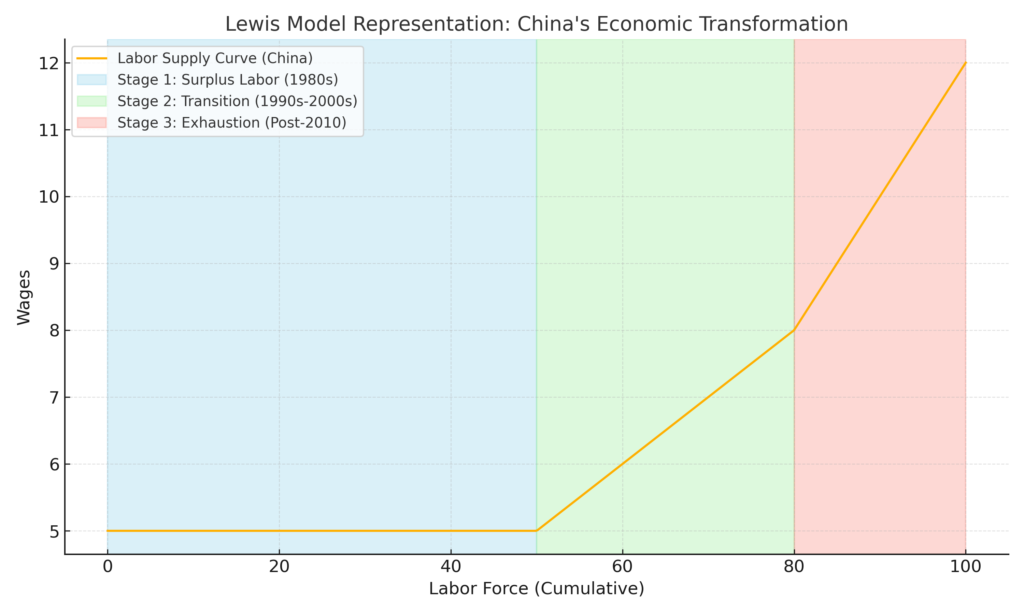
Ques 2: Read the FT article on China. Illustrate the Lewis model using the Chinese situation (use graphs preferably). Which factor(s) were responsible for the armies of surplus labour in the early part of the period considered in the article and how did these factors change over the period?
Answer. A brief summary: There were productivity enhancements as a result of the reforms by Deng Xiaoping. Farm output soared in the 1980s though mechanisation and, hence, productivity gains were limited. As a result, agricultural wages were low and industrial wages did not have to be very high to induce people to move. Such asituation approximates conditions described by the 1st stage of the Lewis model. There is surplus labour in agriculture so there is a ready supply of food and labour for industry. Profits are ploughed back into industry leading to growth. This continues till the third phase which in China has come earlier, because it exhausted its population advantage due to one child policy. In this phase the marginal product in agriculture is as high as industry so wages between the two sectors converge. To grow further China needs more technological improvements in the manufacturing sector to reduce dependence on labour. Moreover, China has become a net importer of food. Without trade, it would be hard to sustain low food output with massive industrialization.
1. Early Stage: Surplus Labor in Agriculture
- Factors Responsible for Surplus Labor:
- Collectivized Farming: Before reforms, inefficiencies in the collective farming system resulted in significant underemployment and low productivity in agriculture.
- Large Rural Population: A significant portion of China’s population lived in rural areas, creating a pool of surplus labor with low marginal productivity.
- Limited Mechanization: Agricultural methods were labor-intensive, and mechanization was minimal.
- Reforms and Transition:
- Deng Xiaoping introduced the Household Responsibility System, increasing farm productivity by allowing farmers to retain profits.
- Agricultural Output Soared: While output increased, mechanization remained limited, maintaining surplus labor in the sector.
- Industrial Sector Growth: Surplus agricultural labor began moving into urban industries, where wages, though low, were higher than subsistence-level agricultural wages.
2. Middle Stage: Rapid Industrial Growth
- Characteristics:
- Surplus labor from rural areas continued to supply the growing industrial sector.
- Industrial profits were reinvested into further expansion, aligning with the Lewis Model.
- Agricultural productivity increased moderately but remained below industrial productivity, ensuring continued migration.
- Wage Dynamics:
- Industrial wages were low but sufficient to attract rural labor due to low agricultural wages.
- Food supply remained stable, supported by rural productivity and imports.
3. Late Stage: Exhaustion of Surplus Labor
- Factors Leading to Exhaustion:
- One-Child Policy: Implemented in the 1980s, this policy reduced the growth of the working-age population, depleting the labor pool faster.
- Urbanization: By the mid-2000s, a majority of surplus rural labor had already migrated to cities, leaving fewer workers in agriculture.
- Rising Wages: As surplus labor disappeared, wages in both the agricultural and industrial sectors began to converge, reflecting the third phase of the Lewis Model.
- Challenges:
- Agricultural productivity plateaued, and China became a net importer of food, reducing the ability of the domestic agricultural sector to support industrial expansion.
- Future growth now depends on technological innovation and productivity gains in manufacturing, as labor-intensive growth is no longer sustainable.
Ques 3: It is unrealistic to assume that farmers voluntarily keep their consumption of food grains the same after migration takes place. Discuss some policies that countries have used historically that are consistent with this Lewis model assumption?
Answer (based on DR, Ch. 10, p. 367-372):
- Agricultural taxation: Industrial sector prefers that agricultural incomes stay low to encourage migration as well as keep the price of food low. Otherwise, if consumption in agriculture increases, the price of food grains on the market reduces leading to higher nominal wages for workers in industry. Cons of this policy: may be easy to evade taxes and requires a lot of information. Land taxes is another possibility – difficult to evade if land ownership records are available. Lobbying by large landowners would prevent this.
- Agricultural pricing policy: output price controls or input subsidisation. Output prices can be capped but would have long term implications for production incentives (but so does tax). Provide incentives to farmers to produce more such as support prices to insure against downturns – where does the subsidy come from? Who pays these taxes? Keeping export prices low by overvaluing exchange rates is another way to do it that is less transparent and therefore more politically feasible.
1. Agricultural Taxation
Description:
- Governments impose taxes on agricultural incomes to suppress consumption in the rural sector, keeping food prices low and facilitating the flow of surplus labor to the industrial sector.
- Low agricultural incomes discourage rural workers from staying in agriculture, making industrial wages relatively attractive.
Historical Applications:
- Soviet Union (1920s–1930s): The state implemented agricultural taxation policies to extract resources from agriculture to fund rapid industrialization.
- China (1950s–1970s): Policies under Mao taxed rural agriculture indirectly through government procurement at below-market prices.
Cons:
- Taxes may be evaded if proper systems (e.g., records of land ownership) are not in place.
- Land taxes could be effective but face resistance from powerful landowners.
- Heavy taxation can lead to reduced agricultural productivity if farmers lack incentives to produce more.
2. Agricultural Pricing Policies
Description:
- Output Price Controls: Governments cap the price of agricultural products to keep food affordable for urban industrial workers.
- Input Subsidies: Farmers are provided subsidies on inputs like seeds, fertilizers, or irrigation to maintain production levels despite lower output prices.
Historical Applications:
- India (Green Revolution, 1960s–1970s):
- Support prices ensured farmers had minimum returns while keeping food prices stable.
- Subsidized fertilizers and irrigation encouraged production.
- Latin America (20th century): Overvalued exchange rates were used to keep export prices of agricultural products low, indirectly controlling domestic prices.
- Japan (Meiji Restoration): Heavy government control of rice prices kept food affordable for urban workers during industrialization.
Cons:
- Price caps can discourage farmers from producing more in the long term, leading to food shortages.
- Subsidies require significant government funding, raising questions about who bears the fiscal burden (urban workers through taxes or deficit financing).
- Overvalued exchange rates reduce export competitiveness, potentially destabilizing the broader economy.
3. Overvalued Exchange Rates
Description:
- Governments maintain an artificially high exchange rate, reducing the price of agricultural exports.
- Farmers receive less income for their produce on the international market, effectively subsidizing urban food prices.
Historical Applications:
- Argentina and Brazil (Mid-20th Century): Used overvalued exchange rates to control food prices in urban areas while promoting industrialization.
- Nigeria (1970s–1980s): Overvalued exchange rates were implemented to lower food costs but eventually led to rural discontent and reduced agricultural output.
Cons:
- Overvaluation benefits urban consumers at the expense of rural farmers, exacerbating rural-urban inequality.
- Prolonged use of this policy can lead to economic distortions, including trade imbalances and reduced export revenues.
Empirical Examples and Outcomes
- China: During the early stages of industrialization under Mao, rural agriculture was heavily taxed to support urban industrial development. Procurement policies and low-price mandates forced farmers to supply grain at low prices, aligning with the Lewis Model’s assumptions.
- India: Green Revolution policies balanced incentives for farmers with low food prices for urban workers, delaying labor market pressures.
- Soviet Union: Collectivization and taxation supported industrial growth but led to widespread rural hardships, including famine.
Key Trade-Offs in Policies
- Encouraging Migration vs. Sustaining Agricultural Production:
- Policies that suppress rural consumption or income can facilitate migration but risk undermining agricultural productivity.
- Short-Term Gains vs. Long-Term Consequences:
- Price controls or overvalued exchange rates may provide short-term benefits for industrial wages but can harm the agricultural sector’s growth and sustainability.
Conclusion
The policies of agricultural taxation, pricing controls, and exchange rate manipulation have historically been used to align with the Lewis model’s assumption of constant rural food consumption. While these policies effectively suppress rural wages and encourage migration, they often come with long-term consequences, including reduced agricultural productivity and heightened rural-urban inequality. Policymakers must carefully balance these trade-offs to sustain both agricultural and industrial growth.

Leave a Reply