An very interesting technical book by Ernmie Chan, ‘Algorithmic Trading : Winning Strategies and Their Rationale’. (Book Notes)

Common Pitfall of Backtesting

Backtesing of the process of feeding historical data to your trading strategy to see how good it have performed.

Look-ahead Bias:

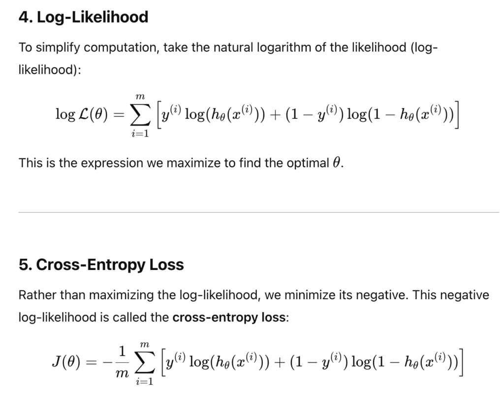
Look-ahead bias means that your backtest program is using tommorrow’s prices to determine today’s trading signals.

A example of look-ahead bias: Use a day’s high or low price to determine the entry signal during the same day during backtesting. (Before the close of a trading day, we can’t know what the high and low price of the day are.)

Look-ahead bias is essentially a programming error and can infect only a backtest program but not a live trading program because there is no way a live trading program can obtain future information.

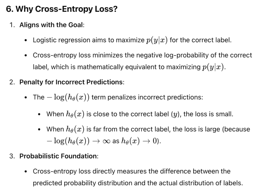
Data Snooping

Practical Implication in Python: Building a Factor-Based Stock Ranking Model

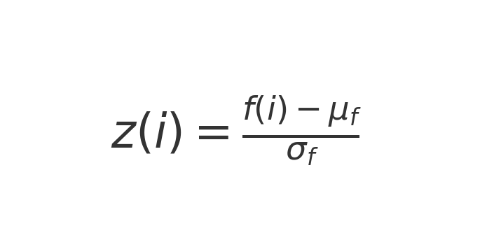
Systematically rank stocks based on multiple predictive factors, standardize these factors using Z-scores, and construct a long-short equity portfolio to exploit the ranking.

Theoretical Explanation

Equal-Weighted Linear Factor Model
- Each factor is standardized using Z-scores to ensure comparability.
- The prediction for returns is a linear combination of these normalized factors, weighted equally but signed according to their correlation with returns.
Robustness of Equal Weights
- Kahneman’s insight suggests that equal-weighted models often outperform more complex models due to robustness against overfitting and sampling errors.
- Equal weighting avoids excessive sensitivity to noise in historical data.
Stock Ranking Instead of Return Prediction
- Instead of predicting returns directly, stocks are ranked based on their factor scores.
- This simplifies the model, focusing on relative performance (ranking) rather than absolute return prediction.
Portfolio Construction
- A long-short portfolio can be created by going long on the top-decile stocks and short on the bottom-decile stocks based on the combined factor ranking.
- This strategy leverages the relative strength of stocks while minimizing market exposure.
Need for Walk-Forward Testing
- To mitigate data-snooping bias, the model must be validated using walk-forward testing or even live trading with small capital to capture real-world constraints like slippage, transaction costs, and market impact.

Python

import pandas as pd
import numpy as np

# Example stock data with two factors: 'factor_1' and 'factor_2'
# For simplicity, we assume a small universe of 10 stocks
np.random.seed(42)
stocks = ['Stock_' + str(i) for i in range(10)]
factor_1 = np.random.normal(0, 1, 10)  # e.g., return on capital
factor_2 = np.random.normal(0, 1, 10)  # e.g., earnings yield

# Combine into a DataFrame
df = pd.DataFrame({
    'Stock': stocks,
    'Factor_1': factor_1,
    'Factor_2': factor_2
})

# Assume Factor_1 positively correlates with returns, Factor_2 negatively correlates
factor_signs = {'Factor_1': 1, 'Factor_2': -1}

# Standardize factors (Z-scores)
for factor in ['Factor_1', 'Factor_2']:
    df[factor + '_Z'] = (df[factor] - df[factor].mean()) / df[factor].std()
    df[factor + '_Adj'] = factor_signs[factor] * df[factor + '_Z']

# Calculate the combined score (equal-weighted)
df['Combined_Score'] = df[['Factor_1_Adj', 'Factor_2_Adj']].mean(axis=1)

# Rank stocks based on combined scores
df['Rank'] = df['Combined_Score'].rank(ascending=False)

# Select long and short portfolios
top_decile = df.nsmallest(2, 'Rank')  # Long top-ranked stocks
bottom_decile = df.nlargest(2, 'Rank')  # Short bottom-ranked stocks

print("Top Decile (Long):\n", top_decile[['Stock', 'Combined_Score']])
print("\nBottom Decile (Short):\n", bottom_decile[['Stock', 'Combined_Score']])

Impact of Stock Splits and Dividend Adjustments on Backtesting

Stock Splits Impact:
- In an N-to-1 stock split, the stock price is divided by N, and the share count increases by N, keeping the total market value unchanged.
- Without price adjustment, a sudden price drop on the split’s ex-date may trigger false trading signals in backtests.
- Adjustment Needed: Divide historical prices before the ex-date by N for forward splits and multiply by N for reverse splits to maintain price continuity.
Dividend Impact:
- On the ex-dividend date, stock prices typically drop by the dividend amount ($d) to reflect the payout.
- Unadjusted price drops in historical data can lead to erroneous signals (e.g., false sell triggers).
- Adjustment Needed: Subtract the dividend amount ($d) from historical prices before the ex-date to smooth out the price series.
Live Trading Consideration:
- These adjustments must also be applied in live trading before the market opens on ex-dates to prevent misleading signals.
Backtesting Accuracy:
- Failing to adjust for splits and dividends skews performance metrics and can result in inaccurate strategy evaluation.
- Proper adjustments ensure that backtests reflect the true economic impact of corporate actions.
ETFs and Options:
- ETFs follow similar adjustment rules for dividends and splits.
- Options pricing requires more complex adjustments due to contract specifications and strike price changes.

Python

# Implementation of Stock Split and Dividend Adjustments for Backtesting
import pandas as pd

# Sample historical stock data (Date, Price, Split Ratio, Dividend Amount)
data = {
    'Date': ['2024-01-01', '2024-01-02', '2024-01-03', '2024-01-04', '2024-01-05'],
    'Price': [100, 102, 98, 50, 51],  # Price drop due to split on 2024-01-04
    'Split_Ratio': [None, None, None, 2, None],  # 2-for-1 split on 2024-01-04
    'Dividend': [0, 0, 1, 0, 0]  # $1 dividend on 2024-01-03
}

df = pd.DataFrame(data)
df['Date'] = pd.to_datetime(df['Date'])

# Adjust for stock splits
for i in range(len(df)):
    if pd.notnull(df.loc[i, 'Split_Ratio']):
        ratio = df.loc[i, 'Split_Ratio']
        df.loc[:i - 1, 'Price'] /= ratio  # Adjust historical prices

# Adjust for dividends
for i in range(len(df)):
    if df.loc[i, 'Dividend'] > 0:
        dividend = df.loc[i, 'Dividend']
        df.loc[:i - 1, 'Price'] -= dividend  # Adjust historical prices

# Final adjusted prices
print("Adjusted Historical Prices:\n", df[['Date', 'Price']])

# This implementation ensures price continuity in backtests by:
# 1. Dividing historical prices by the split ratio before the ex-split date.
# 2. Subtracting dividend amounts from historical prices before the ex-dividend date.

Short-Sale Constraints and Their Impact on Backtesting

Mechanics of Short Selling

To short a stock, brokers must locate and borrow shares from other investors or institutions.
Stocks with high short interest or limited float can become hard to borrow. (Float refers to the number of shares available for public trading (excluding insider holdings, restricted shares, etc.).)
Hard-to-borrow stocks may incur higher borrowing costs or be unavailable for shorting in desired quantities.

Short-Sale Constraints in Backtesting

Backtests often assume unlimited shorting ability, leading to unrealistic performance if hard-to-borrow stocks are included.
Small-cap stocks are more prone to short-sale constraints than large-cap stocks due to lower liquidity.
ETFs can also be hard to borrow, especially during market stress (e.g., SPY after the Lehman Brothers collapse).

Borrowing Costs and Market Impact

Borrowing costs (interest paid to stock lenders) are often excluded from backtests, inflating short-sale profitability.
Limited supply of borrowable shares can cause execution issues or prevent shorting entirely.

Regulatory Constraints

The SEC imposed a short-sale ban on financial stocks during the 2008–2009 crisis, making backtests that ignore this constraint unrealistic.
The Uptick Rule (1938–2007) required shorts to be executed only at a higher price than the last trade to prevent downward price pressure.
The Alternative Uptick Rule (2010–present) activates when a stock drops 10% below its previous close, blocking short market orders during extreme volatility.

Impact on Backtesting Accuracy

Ignoring borrow availability, costs, and regulatory constraints leads to overstated performance in strategies relying on shorting.
Historical data on hard-to-borrow stocks is difficult to obtain, especially since it varies by broker.
Accurate backtests must simulate constraints, including uptick rules, borrow limits, and transaction costs.

Practical Implications for Strategy Development

Backtesting frameworks should include short-selling constraints to reflect real-world limitations.
Applying higher borrowing costs or disallowing shorts on certain stocks can improve realism.
Risk management practices must account for the illiquidity and regulatory risks of short positions.

Challenges with Futures Continuous Contracts in Backtesting

1. Nature of Futures Contracts

Futures contracts have expiration dates, so strategies must roll over from one contract to the next (e.g., from the front-month contract to the next).
Rolling over involves selling the expiring contract and buying the next one, which can impact strategy performance.

2. Rollover Decisions and Their Impact

Different rollover strategies (e.g., rolling over 10 days before expiry or on open interest crossover) affect trade timing.
Rolling over introduces price gaps between contracts, leading to incorrect P&L or return calculations in backtesting.

3. Price Gaps and Misleading P&L/Return

The price difference between the expiring contract and the new contract on the rollover day creates a false P&L if unadjusted.
Without adjustment, the backtest incorrectly calculates P&L as q(T+1)−p(T) instead of the correct p(T+1)−p(T).

4. Back-Adjustment Methods

Price Back-Adjustment: Adjusts historical prices to eliminate price gaps and ensure correct P&L calculations.
- Problem: Incorrect return calculations due to distorted historical prices.
Return Back-Adjustment: Adjusts prices to ensure correct return calculations.
- Problem: Leads to incorrect P&L calculations.

5. Trade-off Between P&L and Return Accuracy

You cannot simultaneously have both accurate P&L and accurate returns with continuous contract data.
Must choose to prioritize either P&L or returns based on the strategy’s focus.

6. Risk of Negative Historical Prices

Price back-adjustments can result in negative prices in the distant past, which can break models and return calculations.
Some vendors add a constant to all prices to prevent negative values.

7. Strategy-Specific Adjustment Needs

Price back-adjustment is necessary for strategies trading spreads (price differences) between contracts to avoid incorrect signals.
Return back-adjustment is essential for strategies based on the price ratio between contracts to maintain correct signals.

8. Vendor-Specific Adjustments

CSI Data: Uses only price back-adjustment with an optional additive constant to prevent negative prices.
TickData: Offers both price and return back-adjustment options but does not prevent negative prices.

9. Impact on Spread and Calendar Spread Strategies

In calendar spreads, small price differences are sensitive to adjustment errors, making accurate back-adjustment critical.
Incorrect back-adjustments can trigger false trading signals in both backtests and live trading.

10. Key Considerations for Backtesting

Understand how the data vendor performs back-adjustments (price vs. return).
Choose the adjustment method that aligns with your strategy (spread-based vs. ratio-based).
Be aware that back-adjustment choices directly impact backtest reliability.

When Not to Backtest a Strategy: Key Points

1. Poor Risk-Adjusted Returns (Low Sharpe Ratio, Long Drawdown)

Example: Strategy with a 30% annual return, Sharpe ratio of 0.3, and a 2-year drawdown.
Issue: High returns may result from data-snooping bias.
Risk: Long drawdowns are emotionally and financially unsustainable.
Action: Avoid backtesting strategies with high returns but low Sharpe ratios and prolonged drawdowns.

2. Underperforming Benchmark Strategies

Example: Long-only crude oil strategy returned 20% in 2007 with a Sharpe ratio of 1.5, while a buy-and-hold strategy returned 47% with a Sharpe ratio of 1.7.
Issue: Strategy underperforms a basic benchmark.
Action: Always compare strategies against appropriate benchmarks (e.g., Information Ratio for long-only strategies).

3. Survivorship Bias in Data

Example: A buy-low-sell-high strategy shows a 388% return in 2001.
Issue: The backtest likely excluded delisted stocks, leading to survivorship bias.
Risk: Ignoring failed companies inflates performance.
Action: Ensure the data used is survivorship-bias-free for realistic backtests.

4. Overfitting in Complex Models (e.g., Neural Networks)

Example: Neural network with 100 nodes achieves a Sharpe ratio of 6.
Issue: Too many parameters result in overfitting to in-sample data.
Risk: Model likely has no predictive power in live trading.
Action: Avoid overly complex models that can fit any dataset but fail to generalize.

5. Limitations of Backtesting High-Frequency Trading (HFT) Strategies

Example: HFT strategy on E-mini S&P 500 with 200% return, Sharpe ratio of 6, and 50-second holding period.
Issue: HFT performance is highly sensitive to execution methods, order types, and market microstructure.
Risk: Backtesting cannot accurately simulate real-time market reactions.
Action: Be skeptical of HFT backtests; real-world trading involves unpredictable dynamics.

6. General Guidelines for Avoiding Wasteful Backtesting

Strategies with high returns but poor risk metrics (e.g., low Sharpe ratio, long drawdowns) are unreliable.
Strategies that underperform basic benchmarks offer no advantage.
Avoid strategies tested on biased data, especially with survivorship bias.
Be cautious of models with excessive complexity prone to overfitting.
Recognize the limitations of backtesting high-frequency and execution-dependent strategies.

Programming Skill Levels and Their Impact on Algorithmic Trading Strategy Development

1. Low Programming Skill: GUI-Based Trading Platforms

Use drag-and-drop interfaces to build strategies without coding.
Examples: Deltix, Progress Apama.
Limitation: Restricted flexibility and customization for complex strategies.

2. Basic Programming Skill: Scripting and Excel-Based Solutions

Use Microsoft Excel with Visual Basic (VB) macros for basic backtesting.
Drawbacks:
- Limited scalability for complex strategies.
- Inefficient performance for data-intensive tasks.
- Requires DDE links for market data integration, making execution cumbersome.
Some platforms (e.g., QuantHouse, RTD Tango) offer proprietary scripting languages that are easier to learn but may still limit strategy complexity.

3. Intermediate Programming Skill: REPL Scripting Languages (Python, R, MATLAB)

Python, R, and MATLAB are ideal for backtesting due to:
- Ease of debugging and interactive development (REPL: Read-Eval-Print Loop).
- High flexibility and efficiency for handling large datasets.
- Simple handling of data types (scalars, arrays, strings).
MATLAB can integrate with Java, C++, and C# for computationally intensive tasks.
Broker APIs for Execution:
- MATLAB: Connects to brokers via Datafeed Toolbox, IB-Matlab, quant2ib, and MATFIX.
- Python: Uses IbPy to connect to Interactive Brokers.
- Open-source solutions like QuickFIX for FIX protocol connectivity.

4. Advanced Programming Skill: General-Purpose Programming Languages (Java, C++, C#)

Direct implementation of both backtesting and live execution.
Highest flexibility, efficiency, and performance for complex algorithms.
All major brokers offer APIs in these languages or support FIX protocol for trading.
Example: QuickFIX (supports C++, C#, Python, Ruby).
Drawback: Requires in-depth programming knowledge and handling of complex broker connections.

5. Integrated Development Environments (IDEs) and Hybrid Platforms

Many specialized trading platforms now offer IDE-like environments with coding capabilities.
Examples: Deltix, Progress Apama, QuantHouse, RTD Tango.
Combine graphical interfaces with advanced coding support for strategy flexibility.

6. Key Considerations for Choosing a Platform

Execution Complexity: Integration with broker APIs requires more programming skill.

Beginners: GUI-based or simple scripting tools for ease of use.

Intermediate Users: Python, R, or MATLAB for flexible backtesting and execution.

Advanced Users: C++, Java, C# for full control and optimal performance.

What about high(er)-frequency trading? What kind of platforms can support this demanding trading strategy?

The surprising answer is that most platforms can handle the execution part of high-frequency trading without too much latency (as long as your strategy can tolerate latencies in the 1- to 10-millisecond range), and since special-purpose platforms as well as IDEs typically use the same program for both backtesting and execution, backtesting shouldn’t in theory be a problem either.

Understanding High-Frequency Trading (HFT) and Platform Limitations

1. Sources of Latency in High-Frequency Trading

Live Market Data Latency:
- Requires colocation at the exchange or broker’s data center for 1–10 ms data delivery. _{(Colocation in trading refers to the practice of placing a trader’s computers or servers in the same data center or in close proximity to a stock exchange or brokerage’s servers to significantly reduce latency in trade execution.)}
- Direct data feeds (e.g., from NYSE) are faster than consolidated feeds (e.g., SIAC’s CTS). _{[SIAC CTS stands for the Securities Industry Automation Corporation Consolidated Tape System. It is a system used to consolidate and distribute real-time trade data for securities traded on major U.S. stock exchanges.]}
- Example: Interactive Brokers offers data snapshots every 250 ms, which is too slow for HFT.
Brokerage Order Confirmation Latency:
- Retail brokers can take up to 6 seconds to confirm order execution.
- Delays impact limit order strategies that depend on quick confirmation.

2. Colocation Strategies to Reduce Latency

Cloud Servers (VPS):
- Reduce risks from power/internet outages but may not improve data latency.
- Latency depends on physical proximity to the broker/exchange.
Data Centers Near Exchanges:
- Providers like Equinix and Telx offer servers close to exchanges for lower latency.
Broker Colocation:
- Hosting trading programs inside broker data centers ensures faster data access.
- Brokers like Lime Brokerage and FXCM provide colocation services.
Exchange Colocation:
- Direct server placement at the exchange or ECN offers the lowest latency.
- Requires a prime broker relationship and large capital due to high costs.

3. Security Concerns with Remote Servers

Intellectual Property Risks:
- Storing algorithms on remote servers may expose them to theft.
Mitigation:
- Upload only executable files (e.g., .p files for MATLAB) instead of source code.
- Use time-based passwords to secure program access.

4. Multithreading in High-Frequency Trading Platforms

Multithreading:
- Essential for trading multiple symbols without delays.
- Java and Python have native multithreading capabilities.
- MATLAB requires the Parallel Computing Toolbox, limited to 12 threads.
No Data Loss in MATLAB:
- MATLAB handles multiple tick listeners without missing data, though with slower processing.

5. Backtesting Challenges for High-Frequency Strategies

Massive Data Handling:
- High-frequency strategies generate huge data volumes (bid/ask, tick data, Level 2 quotes).
- Most platforms struggle with efficiently processing this data.
Execution Dependency:
- HFT performance depends on order types, market microstructure, and other participants’ behavior.
- Backtests often fail to capture these real-time complexities.
Custom Solutions Needed:
- Writing a custom stand-alone program is often necessary for realistic HFT backtesting.

6. Challenges with News-Driven Trading Strategies

Limited News Feed Integration:
- Few platforms support machine-readable news feeds for event-driven trading.
- Progress Apama and Deltix support feeds like Dow Jones, Reuters, and RavenPack.
Expensive API Access:
- Real-time news APIs (e.g., from Reuters, Dow Jones) are costly but essential for news-based HFT.
- Affordable alternatives like Newsware exist for non-HFT strategies.

Complex Event Processing (CEP) in Trading Platforms

1. Definition of Complex Event Processing (CEP)

CEP enables programs to instantaneously respond to market events (e.g., new tick data, news events).
Emphasizes an event-driven model rather than a bar-driven model (which reacts after set intervals like minute/hour bars).

2. CEP vs. Traditional Event Handling

Callback Functions: Basic APIs from brokers can trigger actions when new data arrives but are limited to simple rules.
CEP Systems: Handle complex, multi-layered conditions (e.g., combinations of price movements, order flow, volatility, and news events).
CEP can process intricate rules involving timing clauses like during, between, afterwards, and in parallel.

3. Advantages of CEP

Instantaneous Reactions: No delay between event detection and response.
Simplified Rule Implementation: Easier to express complex strategies using CEP languages compared to traditional programming.
Efficient for Multi-Condition Strategies: Ideal for rules requiring analysis of multiple, time-dependent market signals.

4. Limitations of CEP

Complexity vs. Simplicity Debate:
- Critics argue that complex rules may lead to data-snooping bias.
- CEP advocates claim they’re implementing rules already validated by experienced traders.
Learning Curve: CEP languages may require additional learning compared to familiar programming languages.

5. Examples of CEP in Trading Platforms

Progress Apama: Known for its advanced CEP technology, ideal for real-time event processing.
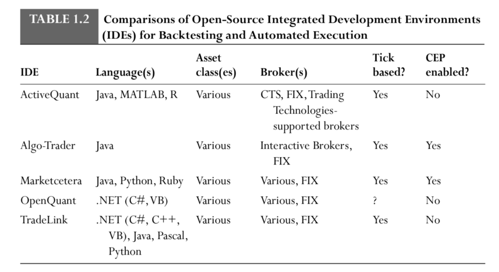
Open-Source IDEs: Some free platforms also support CEP (as mentioned in the text, see Table 1.2).

6. Practical Applications of CEP in Trading

High-Frequency Trading (HFT): Rapid reaction to market events.
News-Driven Strategies: Instant trading decisions based on news sentiment analysis.
Multi-Condition Strategies: Combining technical indicators, order flow, and external data for trade execution.

Mean Reversion in Nature, Social Sciences, and Financial Markets

1. Mean Reversion in Nature

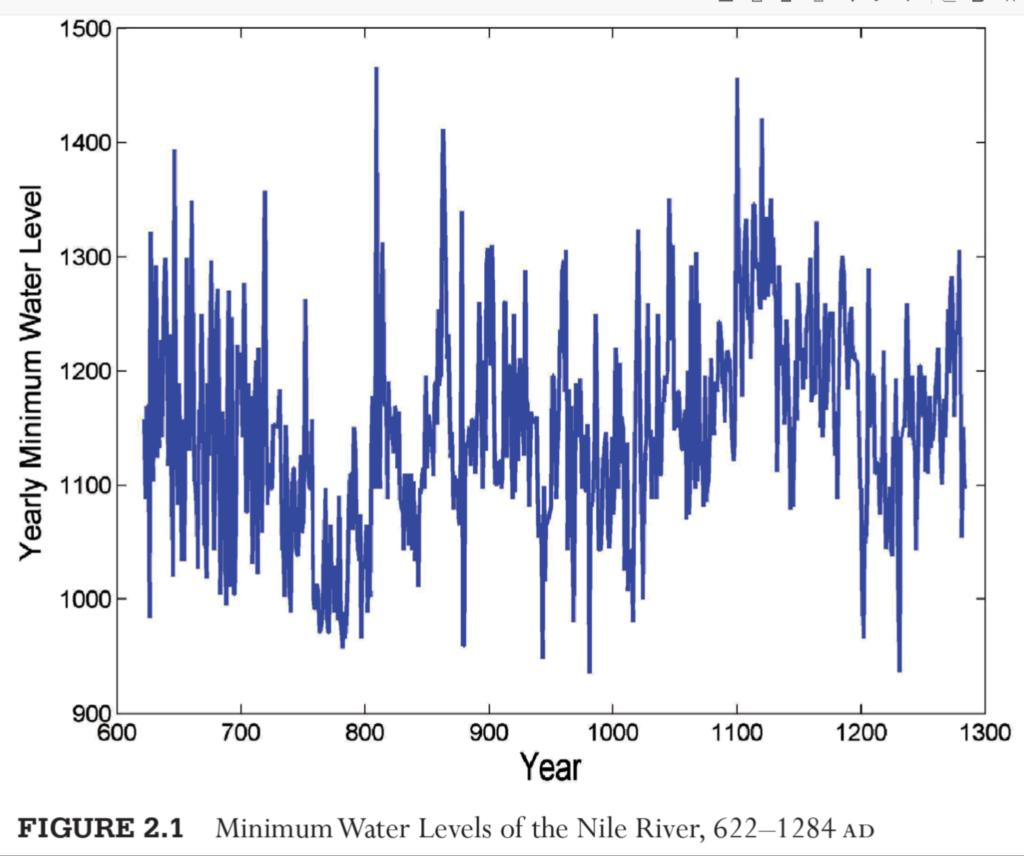
Example: The water level of the Nile River (622 AD to 1284 AD) shows a clear mean-reverting pattern.
Natural systems often fluctuate around a long-term average due to equilibrium-seeking forces.

2. Mean Reversion in Social Sciences

Example: The “Sports Illustrated Jinx” (Daniel Kahneman, 2011).
- Athletes with exceptional performance one year (earning a magazine cover) often regress to their average performance in the following season.
- This is due to random performance variations around a personal performance mean.

3. Mean Reversion in Financial Markets

Mean Reversion in Prices:
- Traders hope that financial prices will revert to a mean level, allowing them to buy low and sell high.
- However, most financial price series follow a geometric random walk rather than mean-reversion.
Mean Reversion in Returns:
- Returns tend to fluctuate randomly around a mean of zero, but this is not directly tradable.
- Anti-serial correlation of returns (negative autocorrelation) is tradable and is equivalent to the mean reversion of prices.
Stationary Series:
- Financial series that revert to the mean are called stationary.
- Statistical tests for stationarity include:
  - Augmented Dickey-Fuller (ADF) Test
  - Hurst Exponent
  - Variance Ratio Test

4. Cross-Sectional Mean Reversion

Occurs when the relative returns of instruments within a basket of assets revert to the basket’s average return.
Implies that the short-term relative returns of assets are serially anti-correlated.
This phenomenon is common in stock baskets and ETFs, and strategies exploiting it will be discussed in more detail later.

5. Practical Challenges in Trading Mean Reversion

If financial markets were broadly mean-reverting, profit-making would be easy.
Most financial assets do not exhibit strong mean-reverting behavior.
Traders must carefully test for stationarity before building strategies around mean reversion.

Mean Reversion and Stationarity in Financial Time Series

Brief Introductions

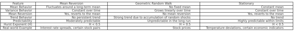
1. Relationship Between Mean Reversion and Stationarity

Mean Reversion and Stationarity describe similar behaviors but focus on different properties of a price series.
A mean-reverting series has future changes that are proportional to the difference between the current price and its mean.
A stationary series has a variance that grows slower than linearly over time, unlike a geometric random walk.

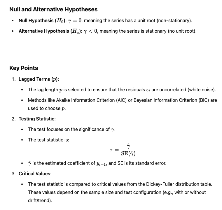
2. Statistical Tests for Mean Reversion and Stationarity

Augmented Dickey-Fuller (ADF) Test:
- Detects if a time series is mean-reverting by checking whether past price levels predict future price changes.
- Tests the null hypothesis that the proportionality constant (λ) is zero (random walk).
- If the null is rejected, the series is mean-reverting.
- The test statistic is λ/SE(λ); it must be negative and lower than the critical value to reject the null.
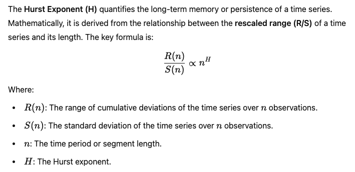
Hurst Exponent (H):
- Measures the rate at which variance grows over time.
- H<0.5 indicates a mean-reverting (stationary) process.
- H=0.5 suggests a random walk (non-stationary).
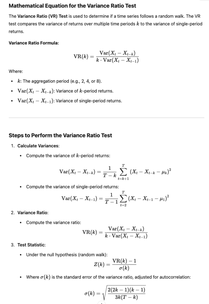
Variance Ratio Test:
- Evaluates if the Hurst exponent equals 0.5 (null hypothesis of a random walk).
- Rejecting the null suggests the series may be mean-reverting or trending.

3. Comparison of Mean Reverting and Stationarity

Mean-Reverting Model:
- Price change depends on how far the price is from its mean.
- If λ≠0, the series is not a random walk and exhibits mean reversion.
- Expressed as:

Stationary Series Behavior:
- The variance grows sublinearly over time, modeled as τ^2H, where:
  - τ = time interval.
  - H = Hurst exponent.
- Sublinear variance growth is a hallmark of stationarity.

Hurst Exponent (H)	Behavior	Best Trading Strategy
H < 0.5	Mean-reverting	Contrarian/Statistical Arbitrage (Buy low, sell high)
H = 0.5	Random walk	No predictable strategy works reliably
H > 0.5	Trend-following	Momentum/Trend-following (Buy high, sell higher)

4. Key Concepts in Practical Trading

Mean Reversion Trading:
- Buy when the price is below the mean, and sell when it returns to the mean.
- The ADF test helps determine if such a strategy is valid for a given asset.
Stationary vs. Non-Stationary Series:
- Stationary series are better suited for mean-reversion strategies.
- Non-stationary series (random walks) are more appropriate for trend-following strategies.
Simplifying Assumptions in Practice:
- Often, the drift term (β) is assumed to be zero because it is small compared to daily price fluctuations.

The Argumented Dickey-Fuller Test (ADF)

If price series is mean reverting, then the current price level will tell us something about what the price’s next move will be. If the price level is higher than the mean, the next move will be a downward move. The ADF is just based on this observation.

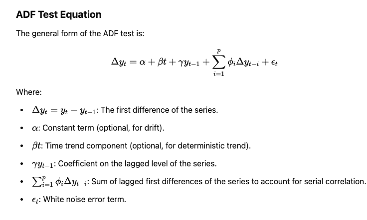
The ADF test will find out whether γ = 0, if the hypothesis γ = 0 can be rejected, that means the next move Δy_t will depend on the current level y_(t-1) , and therefore not a random walk.

If a unit root exists, the lag coefficient(γ) equals 1, meaning past information persists indefinitely, shocks are permanent, and the series is non-stationary, relying entirely on accumulating random noise.

When the lagged coefficient is greater than 0 and less than 1, the series is stationary, mean-reverting, with past effects decaying exponentially, and has finite, stable variance over time.

When the lagged coefficient is zero, the series is pure white noise, entirely random, stationary, with no dependence on past values, and driven only by independent random shocks.

Since we expect mean regression, the DF statistics has to be negative, and it has to be more negative than the critical value for the hypothesis to be rejecyed. The critical values themselves depend on the sample size and whether we assume that the price series has a non-zero mean or a steady drift.

In practical trading, the constant drift in price tends to be of a much smaller magnitude than the daily fluctuation in price. So for simplicity we will assume this drift term to be zero (β = 0)

β > 0: A positive drift indicates an upward trend, suggesting that the series increases on average over time.
β < 0: A negative drift indicates a downward trend, meaning the series decreases on average over time.
β = 0: No deterministic trend; the series changes purely due to random noise and other dynamic factors.

Python Implementation of the ADF Test for Mean Reversion

Let’s implement the ADF test on a time series (like USD/CAD) using Python with the statsmodels library.

Step 1: Connect to the Interactive Broker API

Make sure you download a the Trader Workstation. Launch it and make sure you enable the API at the configuration in the setting.

Open your IDE, and make sure you download the required modules, and import them:

Python

import pandas as pd
import numpy as np
from statsmodels.tsa.stattools import adfuller
import matplotlib.pyplot as plt
from ib_insync import *
import nest_asyncio

nest_asyncio.apply()

After this, you should connect to the Interactive broker to get access to the real time market infomration.

Python

# Connect to Interactive Broker API
ib = IB()
try:
    ib.connect('127.0.0.1', 7497, clientId = 5)
    print("Connected to IB")

except Exception as e:
    print(f'Error connecting to IB server: {e}')
# Fetching and Processing Market data

After the IB is connected, we can required market price for the USDCAD, here I also asked the IB for the AUDUSD price, this is for our next strategy on the cross currency pairs trade.

Notice that for paper trading account, we normaly can access to up to 1 year of daily prices. Hence, we will require the data three times, each for a single year of data and we will link them in a timely sequence.

Python

# Function to create Forex contract
def get_currency_contract(pair):
    return Forex(pair)

# Function to fetch historical data
def fetch_historical_data(contract, duration, bar_size, end_time=''):
    """Fetch historical data for a given contract."""
    bars = ib.reqHistoricalData(
        contract,
        endDateTime=end_time,
        durationStr=duration,
        barSizeSetting=bar_size,
        whatToShow='MIDPOINT',
        useRTH=False,
        formatDate=1
    )
    df = util.df(bars)  # Convert to Pandas DataFrame
    df['date'] = pd.to_datetime(df['date'])  # Ensure 'date' column is datetime
    df.set_index('date', inplace=True)  # Set 'date' as the index
    return df

# Function to combine historical data
def combine_historical_data(years, contract, bar_size='1 day'):
    """Combine historical data into a single dataframe."""
    combined_data = pd.DataFrame()
    end_time = ''  # Start with the most recent data

    for _ in range(years):
        data = fetch_historical_data(contract, duration='1 Y', bar_size=bar_size, end_time=end_time)
        combined_data = pd.concat([combined_data, data])

        # Update end_time to fetch earlier data
        end_time = data.index.min().strftime('%Y%m%d %H:%M:%S')

    # Remove duplicate entries and sort by date
    combined_data = combined_data[~combined_data.index.duplicated(keep='first')]
    combined_data = combined_data.sort_index()

    return combined_data

# Fetch two currency pair contracts
usdcad_contract = get_currency_contract('USDCAD')
audusd_contract = get_currency_contract('AUDUSD')

# Qualify the contracts
ib.qualifyContracts(usdcad_contract)
ib.qualifyContracts(audusd_contract)

# Fetch historical data for the past 3 years
usdcad_data = combine_historical_data(years=3, contract=usdcad_contract)
audusd_data = combine_historical_data(years=3, contract=audusd_contract)

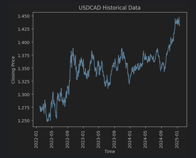
After we stored all the time series price data in the dataframe, we will plot a simple historical price chart to see if there is a mean reverting before going indepth doing a ADF test.

Python

"""
Looking at the price trend, whether there is mean reversion for USDCAD?
"""
print(usdcad_data_1.describe(),
usdcad_data_2.describe(),
usdcad_data_3.describe(),
usdcad_data.describe())
plt.figure()
plt.plot(usdcad_data.index, usdcad_data['close'])
plt.xlabel('Time')
plt.xticks(rotation=90)
plt.ylabel('Closing Price')
plt.title('USDCAD Historical Data')
plt.show()

Here is the historical price chart after running the code. As you see there seems like the price seems to be mean reverting at 1.350. But we should do a ADF test to proof this is actually a mean reversion.

To run the ADF test, be aware the auto lag method you choose, which is the information criterion you are going to use. Different choices will influence the test statistics. (BIC, AIC).

Difference Between BIC and AIC

Both AIC (Akaike Information Criterion) and BIC (Bayesian Information Criterion) are used for model selection, specifically to choose the optimal lag length in the context of the Augmented Dickey-Fuller (ADF) test. Here’s how they differ:

AIC (Akaike Information Criterion):

AIC = −2ln⁡ (Likelihood) + 2k

Likelihood: Reflects the model’s goodness of fit.
k: Number of parameters in the model.
Key Characteristics:
- AIC penalizes complexity, but less so compared to BIC.
- Prioritizes fit over simplicity, so it tends to select models with more parameters.
- Suitable when overfitting is less of a concern.

BIC (Bayesian Information Criterion):

BIC = −2ln⁡ (Likelihood) + kln⁡(n)

nnn: Number of observations.
kkk: Number of parameters.
Key Characteristics:
- BIC penalizes complexity more strongly than AIC, especially with larger datasets.
- Prefers simpler models, making it less prone to overfitting.
- Often used when simplicity and parsimony are priorities.

Which Should You Use in ADF?

BIC: Preferable if you want to ensure a simpler model with fewer lags (avoiding overfitting).
AIC: Preferable if you are prioritizing capturing all potential relationships in the data.

Python


result = adfuller(usdcad_data['close'], maxlag = None, regression = 'c', autolag = 'BIC')

adf_stats = result[0]
p_value = result[1]
used_lag = result[2]
n_obs = result[3]
critical_values = result[4]
ic_best = result[5] # Information Criterion value

# Print results
print("ADF Statistic:", adf_stats)
print("p-value:", p_value)
print("Used lag:", used_lag)
print("Number of observations:", n_obs)
print("Critical values:", critical_values)
print("Information Criterion (if autolag):", ic_best)

# Check stationarity based on p-value
if p_value < 0.05:
    print("The series is stationary (reject the null hypothesis of a unit root).")
else:
    print("The series is not stationary (fail to reject the null hypothesis of a unit root).")

After running the test of the data from historical past three years data on USD.CAD data. The ADF test indicates the price series is not stationary. (Time running this test: 2025, 1, 21). Here is the ADF test result:

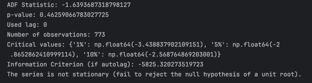
As you see, it failed to reject the Null Hypothesis. THE ADF test statistics is about -1. 64, which is above the critical value at 90% level at -2.57.

In other words, we can’t show that USD.CAD is stationary, which perhaps is not surprisng, given that the Canadian dollar is know as a commodity currency, while the USD is not. (Canada’s economy relies on the export of commodities, particularly crude oli, natural gases, minerals and agricultural products, hence the value of the CAD tends to correlate with the commodity prices.) However, it doesn’t necessarily mean we should give up trading this price series using a mean reversion model. Because, most profitable trading strategies do not requrie such a higher level of certainity.

We can also use the Hurst exponent to check for the stationarity of the USD.CAD

Hurst Exponent

A ‘stationary‘ price series means that the prices diffuse from its initial values more slowly than a geometic random walk would. Mathematically, we can determine the nature of the price series by measuring this speed of diffusion. The speed of diffusion can be charaterised by the variance:

Hurst Exponent Implementation (Python)

Python

def generalized_hurst_exponent(series, q=2, max_lag=20):
    """
    Compute the generalized Hurst exponent H(q) for a given time series.

    Parameters:
    - series: The time series (1D array or list).
    - q: Order of the moment (default is 2).
    - max_lag: Maximum lag to consider (default is 20).

    Returns:
    - Hurst exponent H(q).
    """
    lags = range(2, max_lag + 1)
    variances = []

    for lag in lags:
        # Calculate |z(t+tau) - z(t)|
        diffs = np.abs(series[lag:] - series[:-lag])
        # Calculate 〈 |z(t+tau) - z(t)|^(2q) 〉
        moment = np.mean(diffs ** q)
        variances.append(moment)

    # Fit log-log plot to find slope
    log_lags = np.log(lags)
    log_variances = np.log(variances)
    slope, _ = np.polyfit(log_lags, log_variances, 1)

    # Generalized Hurst exponent H(q)
    return slope / q

# Load the USD/CAD price series
# Assuming `usdcad_data['close']` is the price series
prices = usdcad_data['close'].values

# Compute log of the series (as in the example)
log_prices = np.log(prices)

# Calculate Hurst exponent for q=2
hurst_exponent = generalized_hurst_exponent(log_prices, q=2)

# Display result
print(f"Hurst Exponent (q=2): {hurst_exponent:.4f}")

# Interpretation
if hurst_exponent < 0.5:
    print("The series exhibits mean-reversion (anti-persistence).")
elif hurst_exponent > 0.5:
    print("The series exhibits persistence (trending behavior).")
else:
    print("The series follows a random walk (H ≈ 0.5).")

Using the same USD.CAD price series in the previous example, we put the time series data into the generalised_hurst_exponent function. We set the order of the moment equal to 2, which raises the absolute difference to the power of 2q, amplifying larger difference for higher q.

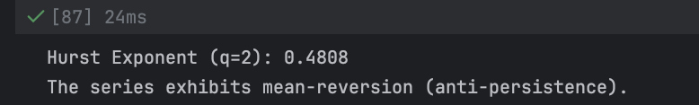
After applying this function, we get H = 0.4808, which means that USD.CAD is weakly mean reverting.

Compute the Half-life for Mean Reversion

After knowning that our strategy is mean reverting (even though only weakly), we know it is possible to profit from the mean-reverting strategy. However, the time it takes to revert to its long-run average also matter, because the longer you hold a position the greater the cost of leverage, rebalancing cost. If the cost is greater than the possible gain from price convergence, it is better not to take this trade.

Python

from statsmodels.api import OLS, add_constant

def calculate_half_life(series):
    """
    Calculate the half-life of mean reversion for a time series.

    Parameters:
    - series: A Pandas Series representing the time series data.

    Returns:
    - halflife: The half-life of mean reversion.
    """
    # Lag the series by 1
    ylag = series.shift(1)

    # Calculate the change in the series (deltaY)
    deltaY = series - ylag

    # Drop NaN values from both deltaY and ylag
    deltaY = deltaY[1:]
    ylag = ylag[1:]

    # Perform linear regression: deltaY = beta * ylag + constant
    X = add_constant(ylag)  # Add a constant to the regression
    model = OLS(deltaY, X).fit()

    # Extract the beta coefficient for ylag
    beta = model.params.iloc[1]

    # Calculate the half-life of mean reversion
    halflife = -np.log(2) / beta

    return halflife


print('The half-life for mean reversion ', calculate_half_life(usdcad_data['close']))

After running the function, the half-life for mean reversion of the USD.CAD is 82.27, which is about 83 days. Depending on your trading horizon, this could be a good strategy in the medium term.

We now, know what look-back to use and what holding period to expect.

A Linear Mean Reverting Trading Strategy

Before develop this strategy:

Ensure you run the DF test to check the price series is indeed mean reverting
Make sure the half-life of mean reversion is short enough to fit in within our trading horizon.

Mean Reversion of Currencies and Futures

Conventional wisdom tells us that currencies and futures are the domain of momentum traders, and conventional wisdom is right about this. Indeed, most CTAs (Commodity trading Advisors) are momentum based.

It is also true that most currency and future pairs would not cointegrate, and most portfolios of currencies or futures do not exhibit cross-sectional mean reversion.

Therefore, opportunities for mean reversion strategies in currencies are limited, but not nonexistent.

Trading Currency Cross-Rates

The basic idea in forming a stationary portfolio of foreign currencies is very similar to the trading of stock index ETF pairs form different countries:

We need to find countries that have similar economic fundamentals
- E.g.: that EWA (Australian stock index ETF) and EWC (Canadian Stock Index ETF) cointegrate with CAD (Canadian dollar) as well.
- Becasue both Australia and South Africa have major mining revenues, we might expect AUD to cointegrate with ZAR (South African rand).
- In fact, trader have called these and other currencies such as the Norwegian Krone commodity currencies.
Trading currency pairs has lots of advantages compared to trading their corresponding stock index ETF pairs.
- Usually, liquidity in currencies is higher (especially for best bid/ask sizes), thus by lowering transaction cost.
- The leverage that can be employed for currencies also much higher
- No short sell-sale constraint for currencies
- Longer Trading Window:
  - At least five days a week;
  - Currency trading starts at 10:00 p.m. GMT (Sunday) and ends at 10:00 p.m. GMT (Friday).

Session	Hours (GMT)	Key Markets
Sydney	10:00 p.m. – 7:00 a.m.	AUD, NZD
Tokyo	12:00 a.m. – 9:00 a.m.	JPY, Asian currencies
London	8:00 a.m. – 5:00 p.m.	EUR, GBP, CHF
New York	1:00 p.m. – 10:00 p.m.	USD, CAD, North and South American currencies

Important Overlaps

The most liquid times in currency trading occur during overlaps between major sessions:

London–New York Overlap:
- 1:00 p.m. – 5:00 p.m. GMT
- High liquidity for USD, EUR, GBP, and other major currencies.
Tokyo–London Overlap:
- 8:00 a.m. – 9:00 a.m. GMT
- Moderate liquidity, mostly for JPY, EUR, and GBP pairs.

Currency Trading Mechanism:

If we are trading cross-rate AUD.ZAR, then AUD is called base currency, and ZAR is the quote currency. If AUD.ZAR is quoted at 9.58, it takes 9.58 ZAR to buy 1 AUD. Buying 100,000 AUD,ZAR meaning you are buying 100,000 AUD, while selling 958,000 if ZAR.
- Note that, in reality, few brokers offer AUD.ZAR as cross-rate. So usually we have to buy X units of B.ZAR and sell X units of B.AUD to effectively buy X AUD worth of AUD.ZAR; Where B is a very liquid base currency. (USD or EUR)
- Therefore, everything we just did is a synthetic pair: USD.ZAR / USD.AUD
When we compute the return of a stratehy trading B.Q, we are assuming that the profits are denominated in our local currency (USD for US investors), which may neither be B nor Q.
So for backesting, we need to regularly convert B and Q into our local currency.
- For example: if our local currency is USD, and we have realised profits of X units of ZAR.USD and Y units ZAR.AUD. We need to buy X units of ZAR.USD and Y unit of ZAR.AUD to close the position.
- If we don’t do this regularly, a large significant deviation from our backtest may happen.

Application: Currency pair trade

Key Assumptions

Currencies Traded:
- B1.USD: The first currency pair with USD as the quote currency.
- B2.USD: The second currency pair with USD as the quote currency.
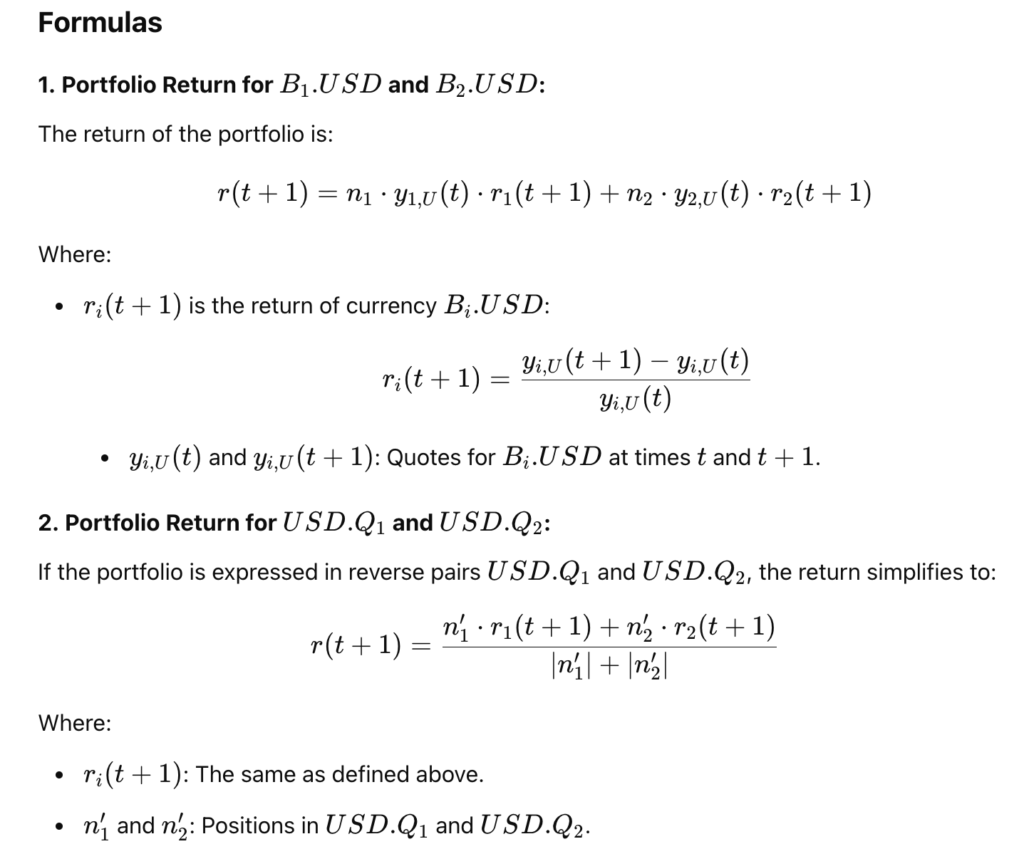
Return of a Portfolio:
- The portfolio consists of n1 units of B1.USD and n2 units of B2.USD.
- The portfolio return is calculated based on the changes in the currency exchange rates.
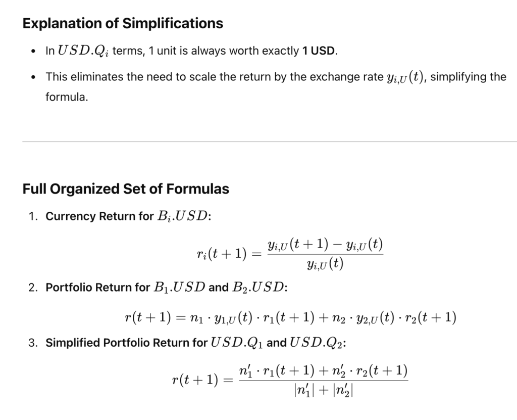
Simplification for Reverse Currency Pairs:
For portfolios expressed in USD.Q1 and USD.Q2, the calculation simplifies because 1 unit of USD.Qi is always worth 1 USD.
Assumption:
Rollover interests (the costs or earnings from holding positions overnight) are ignored here for simplicity.

Python

# Pair Trading USD.AUD versus USD.CAD Using the Johansen Eigenvector

'''
## Concept:
This strategy involves pair trading USD.AUD and USD.CAD with a hedge ratio derived using the Johansen cointegration test. The key steps include:

1. Compute Hedge Ratio: Run the Johansen test on AUD.USD and CAD.USD to derive the hedge ratio.
2. Mean-Reversion Analysis: Use a moving average and standard deviation of the portfolio's market value to identify deviations.
3. Determine Positions: Allocate positions based on the z-score of the deviation.
4. Calculate P&L and Returns: Compute the profit and loss (P&L) and daily portfolio returns.
'''


import numpy as np
import pandas as pd
from statsmodels.tsa.vector_ar.vecm import coint_johansen
from ib_insync import *
import nest_asyncio

nest_asyncio.apply()


# Connect to Interactive Broker API
ib = IB()
try:
    ib.connect('127.0.0.1', 7497, clientId = 5)
    print("Connected to IB")

except Exception as e:
    print(f'Error connecting to IB server: {e}')

# Fetching and Processing Market data

def get_currency_contract (pair):
    return Forex(pair)

# Fetch two currency pair market data from IB
usdcad_contract = get_currency_contract('USDCAD')
usdaud_contract = get_currency_contract('AUDUSD')

# Quantifying the contracts (Ensure they are valid)
ib.qualifyContracts(usdcad_contract, usdaud_contract)

# Request market data
usdcad_ticker = ib.reqMktData(usdcad_contract)
usdaud_ticker = ib.reqMktData(usdaud_contract)

# Allow some time to fetch data
ib.sleep(2)


# Function to fetch historical data
def fetch_historical_data(contract, duration, bar_size, end_time=''):
    """Fetch historical data for a given contract."""
    bars = ib.reqHistoricalData(
        contract,
        endDateTime=end_time,
        durationStr=duration,
        barSizeSetting=bar_size,
        whatToShow='MIDPOINT',  # Options: MIDPOINT, BID, ASK
        useRTH=False,  # Use all available data (not just regular trading hours)
        formatDate=1
    )
    return util.df(bars)  # Convert to Pandas DataFrame

# Fetch historical data for the past 3 years in chunks (1 year at a time)
duration = '1 Y'  # Fetch data 1 year at a time
bar_size = '1 day'  # Daily data

# Fetch data for USDCAD
usdcad_data_1 = fetch_historical_data(usdcad_contract, duration, bar_size)
usdcad_data_2 = fetch_historical_data(usdcad_contract, duration, bar_size, end_time=usdcad_data_1.index[0])
usdcad_data_3 = fetch_historical_data(usdcad_contract, duration, bar_size, end_time=usdcad_data_2.index[0])

# Combine the data for USDCAD
usdcad_data = pd.concat([usdcad_data_3, usdcad_data_2, usdcad_data_1]).drop_duplicates()

# Fetch data for AUDUSD
audusd_data_1 = fetch_historical_data(audusd_contract, duration, bar_size)
audusd_data_2 = fetch_historical_data(audusd_contract, duration, bar_size, end_time=audusd_data_1.index[0])
audusd_data_3 = fetch_historical_data(audusd_contract, duration, bar_size, end_time=audusd_data_2.index[0])

# Combine the data for AUDUSD
audusd_data = pd.concat([audusd_data_3, audusd_data_2, audusd_data_1]).drop_duplicates()



# Remove duplicate indices
audusd_data = audusd_data[~audusd_data.index.duplicated(keep='first')]
usdcad_data = usdcad_data[~usdcad_data.index.duplicated(keep='first')]

# Convert to AUD.USD and CAD.USD
cadusd = 1 / usdcad_data['close']  # Assuming 'close' is the column with prices
audusd = audusd_data['close']

# Align data for AUD.USD and CAD.USD
aligned_data = pd.DataFrame({
    'audusd': audusd,
    'cadusd': cadusd
}).dropna()  # Drop rows with missing values

# Extract aligned data
audusd_aligned = aligned_data['audusd'].values
cadusd_aligned = aligned_data['cadusd'].values

# Combine aligned arrays into a single array (AUD.USD and CAD.USD prices)
prices = np.column_stack([audusd_aligned, cadusd_aligned])

# Parameters
trainlen = 250  # Training period for the Johansen test
lookback = 20   # Lookback for moving average and z-score
hedge_ratios = np.full(prices.shape[0], np.nan)
num_units = np.full(prices.shape[0], np.nan)

# Function to calculate z-score
def calculate_z_score(portfolio, lookback):
    ma = np.mean(portfolio[-lookback:])
    mstd = np.std(portfolio[-lookback:])
    z_score = (portfolio[-1] - ma) / mstd
    return z_score

# Compute hedge ratios and z-scores
for t in range(trainlen, len(prices)):
    # Perform Johansen test
    result = coint_johansen(np.log(prices[t-trainlen:t]), det_order=0, k_ar_diff=1)
    hedge_ratio = result.evec[0, 0] / result.evec[1, 0]
    hedge_ratios[t] = hedge_ratio

    # Portfolio market value
    portfolio = prices[t-lookback:t, 0] - hedge_ratio * prices[t-lookback:t, 1]
    z_score = calculate_z_score(portfolio, lookback)
    num_units[t] = -z_score  # Trading signal based on z-score

# Calculate positions
positions = np.column_stack([num_units * hedge_ratios, num_units]) * prices

# Lag positions and prices
lag_positions = np.vstack([np.zeros((1, positions.shape[1])), positions[:-1]])
lag_prices = np.vstack([np.zeros((1, prices.shape[1])), prices[:-1]])

# Replace zeros in lag_prices with a small value to avoid division by zero
lag_prices = np.where(lag_prices == 0, 1e-10, lag_prices)

# Ensure no NaNs in lag_positions or prices
lag_positions = np.nan_to_num(lag_positions, nan=0.0)
lag_prices = np.nan_to_num(lag_prices, nan=0.0)
prices = np.nan_to_num(prices, nan=0.0)

# Compute P&L and returns
pnl = np.sum(lag_positions * (prices - lag_prices) / lag_prices, axis=1)

# Avoid invalid operations by checking for zero gross market value
gross_market_value = np.sum(np.abs(lag_positions), axis=1)
gross_market_value = np.where(gross_market_value == 0, 1e-10, gross_market_value)

# Calculate returns
returns = pnl / gross_market_value

# Output results
results = pd.DataFrame({
    'Hedge Ratio': hedge_ratios,
    'Num Units': num_units,
    'P&L': pnl,
    'Returns': returns
})

# Remove NaN values (results before sufficient data is available)
clean_results = results.dropna()

print(clean_results)

Johansen Test:

Johansen Test is a statistical test used to determine the presence of cointegration among multiple time series. Cointergration is a concept in time series where two or more non-stationary series have a long-term equilibrium relationship, even though the individual series themselves are non-stationary.

Supervised ML (Inductive learning)

Parametric model assumes a specific variables to be used, a specific form for the underlying data distribution. There a fied number of parameters to define the relationship between input and output variable.

Decision Tree
- non-parametric
- Use: Classification
Linear regression
- para
Linear classifier
- para
- Use: Classification
Logistic regression
- para
- Use: solve classification problem; binary classification
Ensemble method
- can be non or parametric

Pre-requiste of ML model

Loss function
Update Rules

Entropy and Information gain

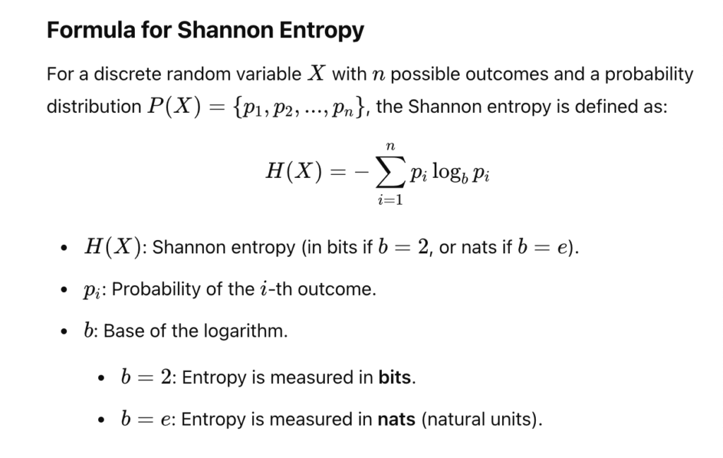
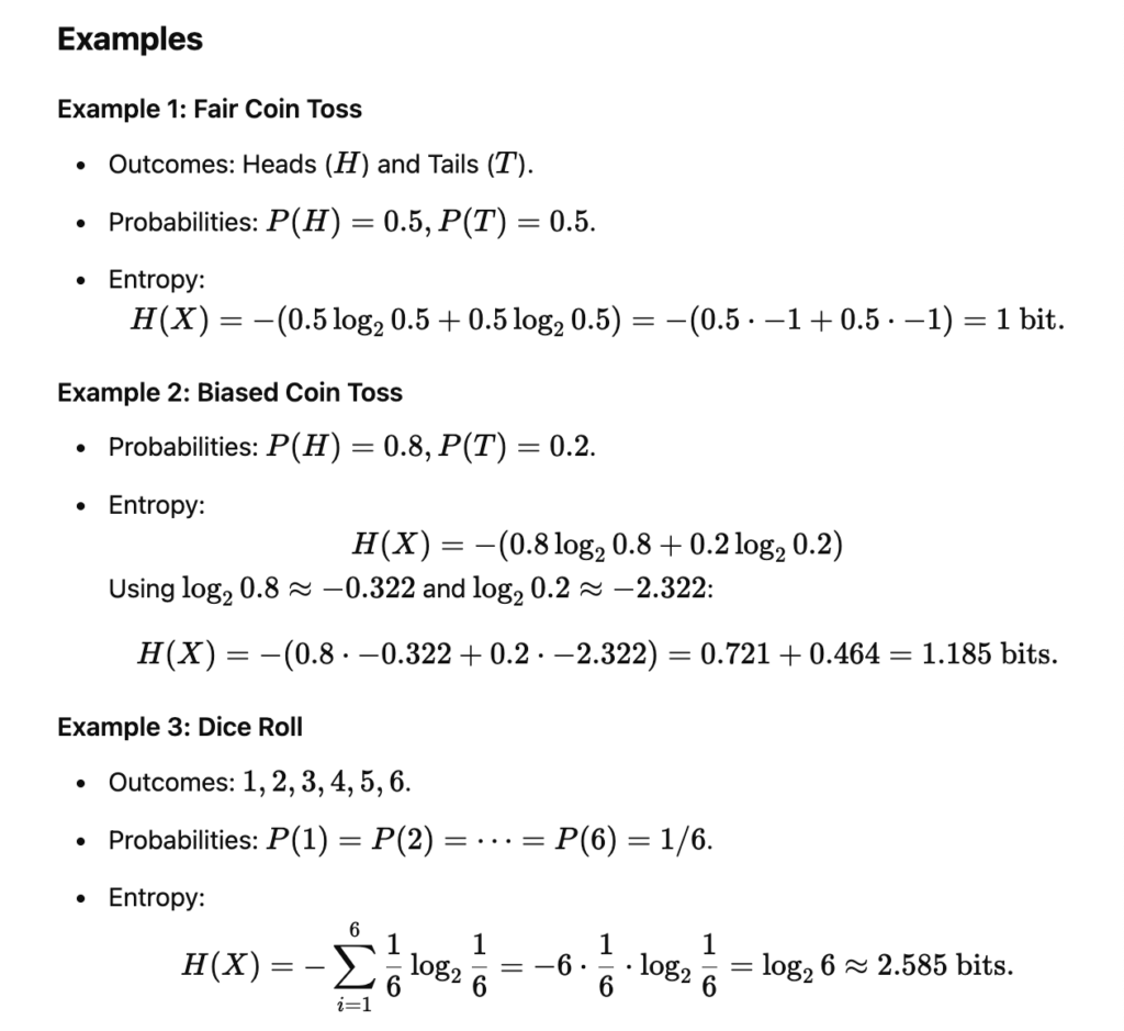
Shannon Entropy: It is the measurment of the uncertainity of a data set; for any balance dataset, the entropy is always going to be 1. It is the weighted average of each node’s uncertainty

Batch gradient descent

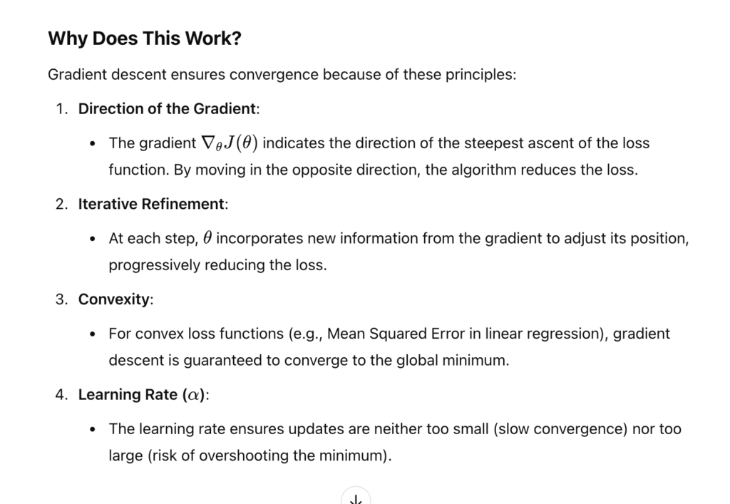
BGD is an optimisation algorithm used to minimise the cost function in machine learning by iteratively updating the model’s parameters. It calculate the gradient of the cost function using the entire dataset for each update of the parameters.

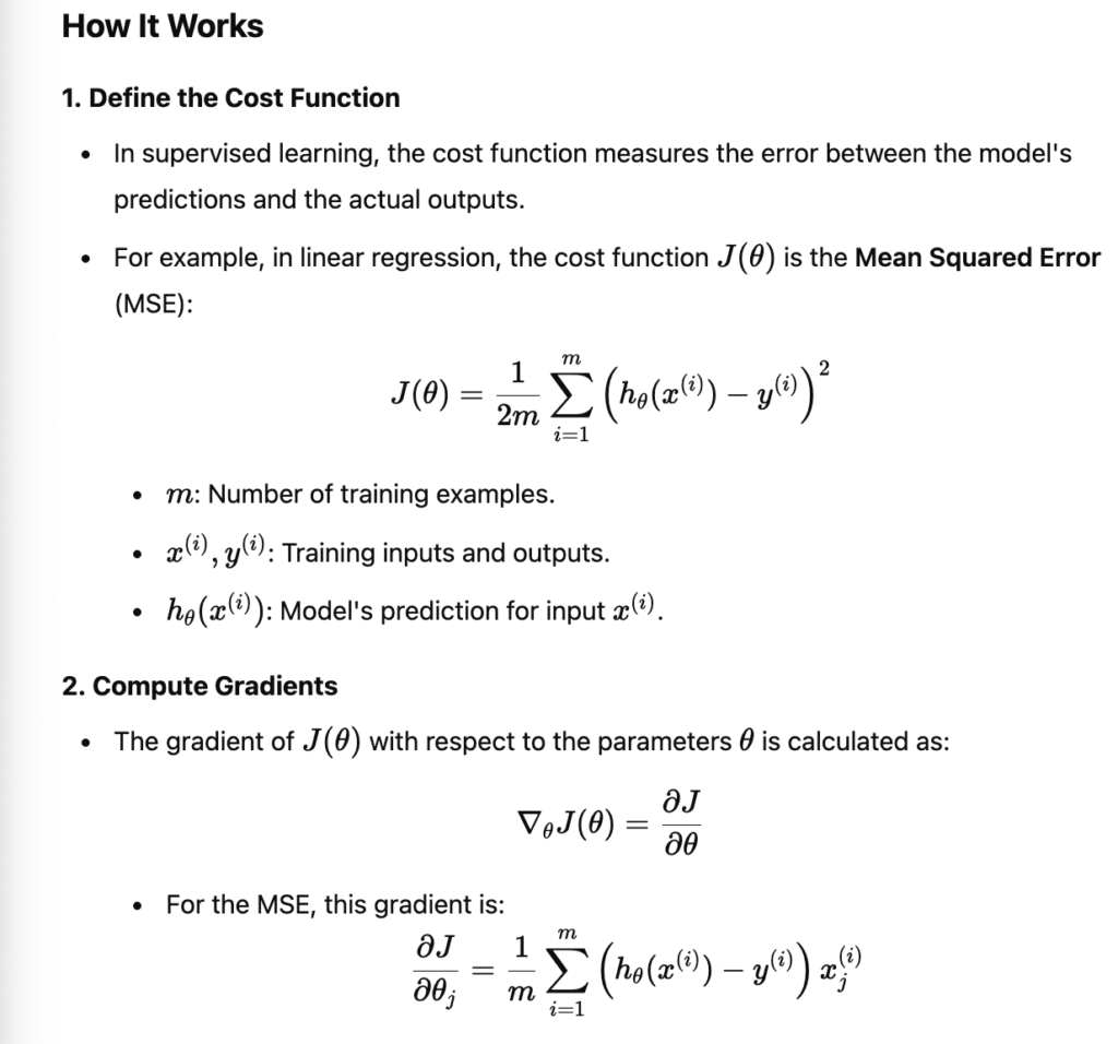
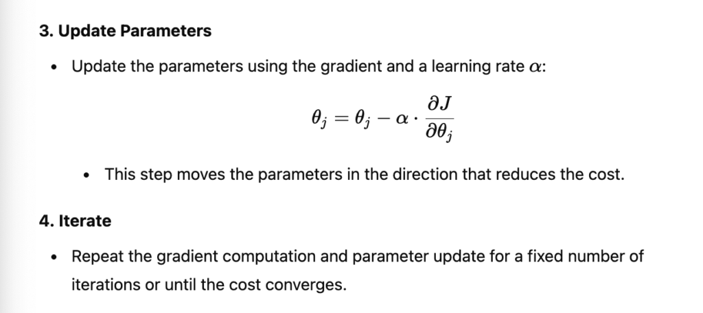
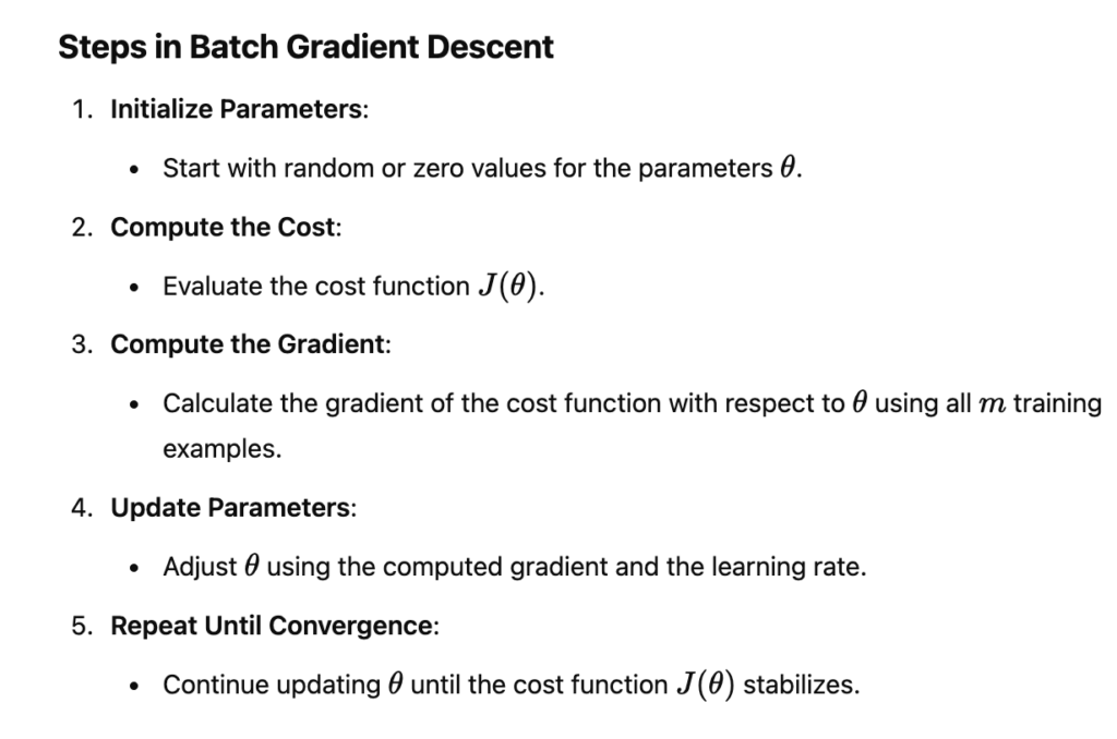
Advantage of BGD

Determinstic Updates:
- The gradients are computed using the entire dataset, so the update are consitent and not noisy
Globla Convergence:
- More stable convergence compared to stochastic approaches
Simplicity:
- Straightforward to implement and analysis

Disad of BGD

Computaionally Expensive: processing the entire dataset for every parameter update can be slow, especially for large datasets.
Money intensive: Requires the entire dataset to be loaded into memory to compute the gradients.
May get stuck in local minima: can converge to suboptimal solutions if the cost function has multiple local minima or plateaus.

Python

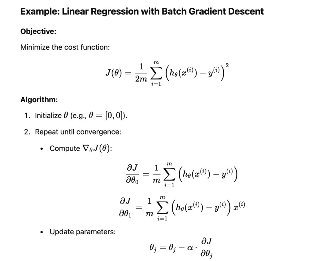
import numpy as np

# Generate sample data
X = np.array([[1], [2], [3], [4]])
y = np.array([2, 4, 6, 8])  # y = 2 * x

# Add bias (intercept) to X
X = np.c_[np.ones(X.shape[0]), X]  # Add column of 1s for the intercept term

# Initialize parameters
theta = np.zeros(X.shape[1])
alpha = 0.01  # Learning rate
iterations = 1000

# Number of examples
m = len(y)

# Batch Gradient Descent
for _ in range(iterations):
    predictions = X.dot(theta)
    errors = predictions - y
    gradients = (1 / m) * X.T.dot(errors) # errors is an array
    theta -= alpha * gradients

print("Learned Parameters:", theta)

Stochastic Gradient Descent

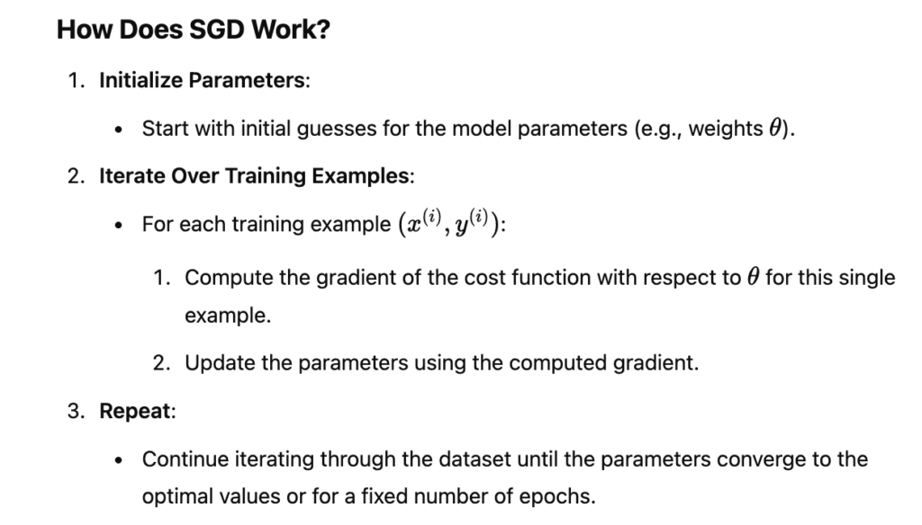
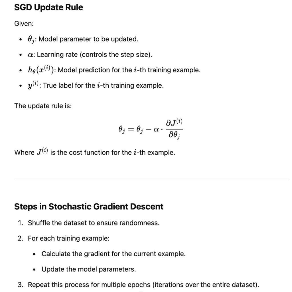
Comparison to Batch Gradient Descent

Feature	Batch Gradient Descent	Stochastic Gradient Descent (SGD)
Gradient Computation	Entire dataset at once.	One training example at a time.
Update Frequency	Updates after processing the entire dataset.	Updates after every example.
Speed	Slower updates due to full dataset computation.	Faster updates (but noisy).
Convergence	Stable but slower.	Faster but may oscillate around minima.
Memory Usage	High (requires entire dataset in memory).	Low (processes one example at a time).

Python

import numpy as np

# Generate sample data
X = np.array([[1], [2], [3], [4]])
y = np.array([2, 4, 6, 8])  # y = 2 * x

# Add bias (intercept) to X
X = np.c_[np.ones(X.shape[0]), X]  # Add column of 1s for intercept term

# Initialize parameters
theta = np.zeros(X.shape[1])
alpha = 0.01  # Learning rate
epochs = 100  # Number of times to iterate through the dataset

# Stochastic Gradient Descent
for epoch in range(epochs):
    for i in range(len(y)):
        # Compute the prediction and error for the current example
        prediction = X[i].dot(theta)
        error = prediction - y[i]
        
        # Compute the gradient for the current example
        # Errors here is an single number
        gradient = error * X[i]
        
        # Update the parameters
        theta -= alpha * gradient

print("Learned Parameters:", theta)

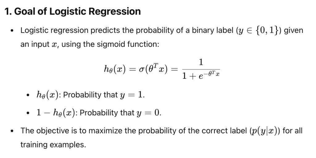
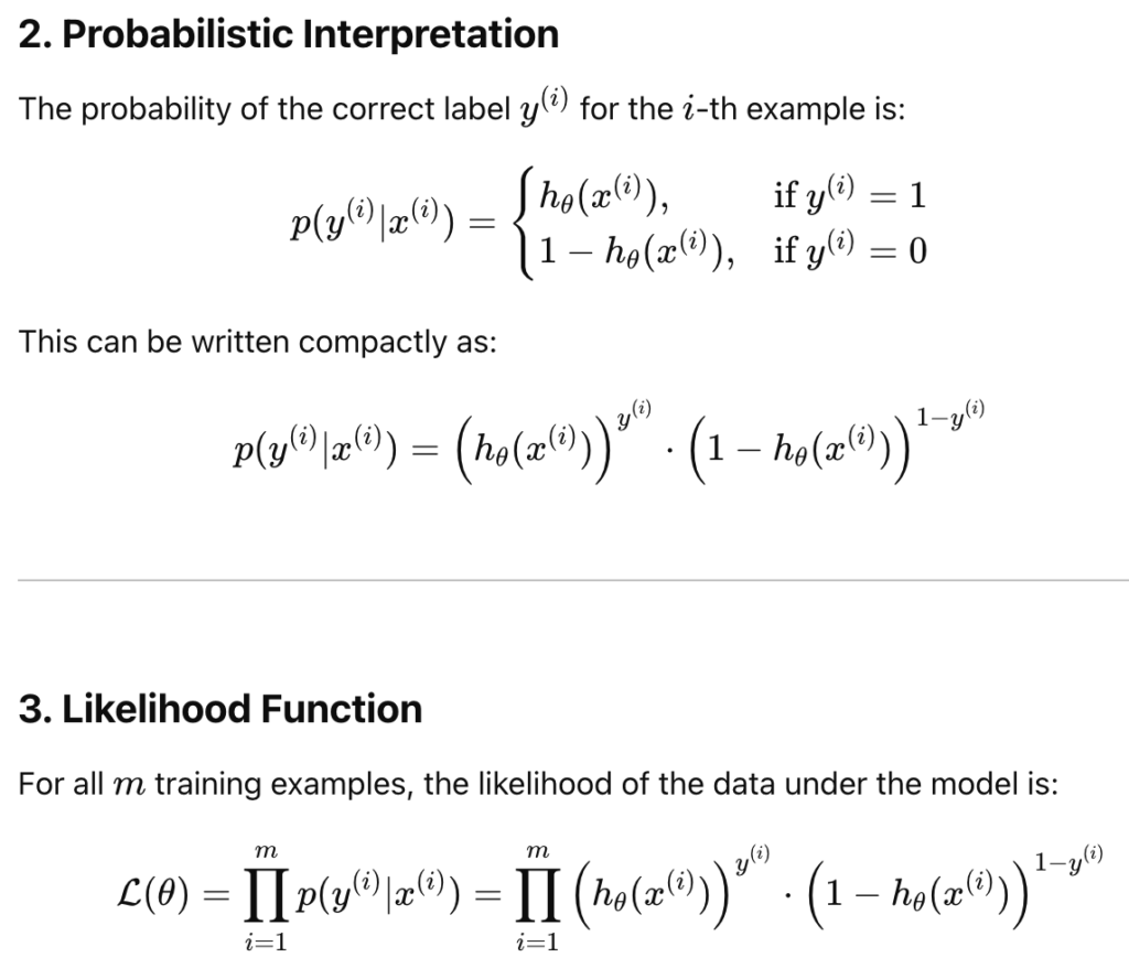
Logistic Regression

logsitic regrression commonly uses the cross-entropy(Shannon Entropy) loss function.
Goal: maximise the probability of the correct label p (y|x)

Python

import numpy as np

# Sigmoid function
def sigmoid(z):
    return 1 / (1 + np.exp(-z))

# Cross-Entropy Loss Function
def compute_loss(y, predictions):
    m = len(y)
    loss = -(1 / m) * np.sum(y * np.log(predictions) + (1 - y) * np.log(1 - predictions))
    return loss

# Gradient Descent Function
def gradient_descent(X, y, theta, learning_rate, epochs):
    m = len(y)  # Number of training examples
    loss_history = []  # To track the loss over epochs
    
    for epoch in range(epochs):
        # Compute predictions
        z = np.dot(X, theta)  # Linear combination
        predictions = sigmoid(z)  # Sigmoid output

        # Compute the gradient
        errors = predictions - y
        gradients = (1 / m) * np.dot(X.T, errors)  # Gradient for each parameter

        # Update parameters
        theta -= learning_rate * gradients

        # Compute and store the loss
        loss = compute_loss(y, predictions)
        loss_history.append(loss)

        # Print loss for every 100 epochs
        if epoch % 100 == 0:
            print(f"Epoch {epoch}, Loss: {loss}")

    return theta, loss_history

# Example Dataset
X = np.array([[1, 2], [1, 3], [1, 4], [1, 5]])  # Features with bias term (column of 1s for theta_0)
y = np.array([0, 0, 1, 1])  # Labels (binary classification)

# Initialize Parameters
theta = np.zeros(X.shape[1])  # Initialize weights as zeros
learning_rate = 0.1
epochs = 1000

# Train Logistic Regression Model
theta, loss_history = gradient_descent(X, y, theta, learning_rate, epochs)

print("\nFinal Parameters (theta):", theta)

High-frequency trading system:

Different ways of order execution:

A trade is placed as an order with a broker’s salesperson who liaise with a trader (or a dealer).
DMA
Intermediary and algo trade
Algo trade
HFT approaches, sponsored access with high speed

Types of trading Strategies:

Common
- Buy-and-hold (long-term)
- Momentum (Trend following)
- Contrarian (Trend reverting)
- Mean-Reversion
High-Freq
- VWAP & TWAP (Volumn, Time weighted average price)
- Pairs Trading
- Statistical Arbitrage
- Event Arbitrage
- Market Making
  - Bid and Ask arbitrage

Trading performance:

peformance analysis:
- P & L
- Accuracy
- Sensitivity
- Implementation
- Shortfall (Difference between the actual and expected trading price)
Cost Analysis
- Subscription fees (Pay for the sponsored access)
- Transaction costs (Pay broker commissions)
- Statistical Arbitrage
- Slippage (negative market price difference, due to high latency)
- Tax
- Opportunity costs

Trader’s dillemma:

Trading signal & optimisation:

Aggressive trading: put the order on the price close to the market price
passive trading: put the order on the limit price far removed from the current market price
all points on the efficient trading frontier are optimal, decisions above are suboptimal
Trading strategy is a trade-off: risk toleranceand cost consideration.

Efficiency trading frontier:(similar market effciency frontier, but instead a trade off between cost and risk)

Aggressive trading (most cost, lower risk)
Passive Trading (higher risk, lower cost)

Risk Management:

Inventory exposure management
Performance monitoring unit
Degree of automation
risk measurement ad risk assessment
exit strategies
capital allocation, levrage and money management

Market model and market microstruture:

Business Structure (Retail or Proprietary)
Market type (Fragmentation)
Asset class
Trading Periods
Liquidity & market volume

Trading platform / System Design

Software Architecture (also: Commercial, APIs, or In-House)
Maintainability & Documentation
Modularity & Coupling
Scalability & Extensibility
Security & Acess Control (Different security level : Entry level or senior level)

Execution Speed(Hardware):

Hardware (e.g: FPGA)
Single-unit or Network (runing on a single computer or multiples)
Distribution & Load Balance (dirtibute computing power evening)
Brokerage or DIrect Market Access (DMA)
Ultra-Low latency (ULL) Technology

Communication Speed(Messaging)

Standards & Protocals:

FIX (Financial Information eXchange)
FAST (FIX Adapted for STreaming)
ITCH and OUCH (Nasdaq’s protocol, faster than FIX)
TCP/IP
UDP

Complexitiy : FIX/ITCH/OUCH > TCP/IP > UDP

Trading Veneue gives quotes: UDP + FIX

TRader trade with trading venue TCP/IP + FIX

Speed vs Security:

Client Server model: SLow, more secure
- traders goes to reliable ISP node
- Then to execution venue
Peer to peer model: faster, less secure
- trader1 may execute trade through trader 2
- trader 2 then pass the trade to the execution venue
co-location mode(for high freq trade):
- trader execute trae with a dedicated network
- no intermediary to the execution venue
- e.g of co-location: london stock exchange

Market Rules:

All electronic trading platforms must have a set of rules that describe the following:

Order Precedence (Priority to orders)
Trade Size (Minimum TRade Quantities)
Price increments (smallest tick size)
Circuit Breakers (TRading Halt Mechanism)

What constitute an order?

Bid order:
- An order submitted by a market partcicipant to purchase an asset.
Ask order:
- an order submitted by a market partcicipant to sell an asset.

Market Order:

Buy or sell at the best available prcie when the order is executed on the market.
Limit order: Allows to set a price limit

Order types:

Stop order: become market order when the price is above the stop price
Stop limit order: become a limited order when the price is above the stop price. Limit order then become a market order, when the limit price is acheived

Other orders:

M2l, GTD, DTK, FOK, AON, IOC

Tick size: The minimum size of an order. Tick size can change over time. If the tick size is large, it may be hard to liquidate the volume.

Limit Order Book:is a trading system operate by a stock exchange for storing and matching the various kind of orders that can be placed on such things.

Order slags

Selling at the bid: hitting the bid

Buying at the offer (lifting the offer)

Trading several buyer or sellers (Walking the book)

Add-one smoothing (aka: Laplace smoothing)

In NB, we compute the conditionals by counting instances. (Books: Murphy; Jurafsky & Martin.)

NB as a baseline:

checking whether our current model does better than an existing approach
the existing approach is refered as a baseline

ML algo choices:

Appropriate algo for task
dumb fast algo or slow complex algo
consistency across datasets

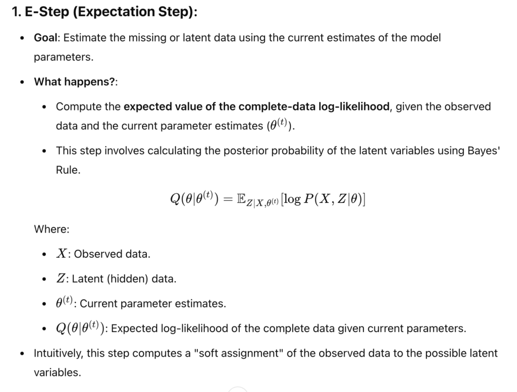
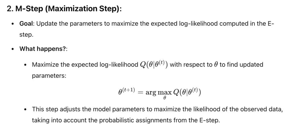
The Expectation-Maximization (EM) algorithm is an iterative method used to find maximum likelihood estimates of parameters in probabilistic models, especially when dealing with incomplete data or latent variables. In the context of probability, the EM algorithm alternates between two steps:

LSE SETs – market model – release 3.1

Everyday trading day, between 7:50 and a random time between 8:00 and 8:00:30, there will be an opening auction during which limit and market orders are entered and deleted on the order book.

At the end of the random start period, the order book is frozen temporalily and an order matching algorithm is run.

A matching price is calculated at whcih the maximum volume of shares can be traded.

Regulation on HFT:

HFTs are required to provide two-sided liquidity on a continous basis. ALl orders will be obligated to stay in the order book for at least 500 milliseconds.

Spread-time priority

queuing uses weigted average between a price and a spread contribution (lower rank, highe priority)

Market maker are encouraged to hold two-sided order; meaning long a security and short the same security at two different price.