In this blog, I will demonstrate how to use python to calculate the price of a call option for the iShares 20+ Years Treasury Bond ETF (Ticker: TLT) using real time data from yfinance.

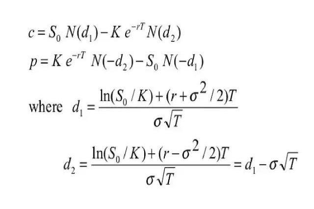
Options are financial derivatives that provide the right, but not the obligation, to buy or sell an asset at a predetermined price. Pricing options accurately is critical for traders, risk managers, and quants. The Black-Scholes model is one of the most popular approaches for calculating the theoretical price of European options.

How does BSM model work?

The Black-Scholes model is defined by two key equations for European call and put options. These equations rely on the assumption that markets are efficient, and the underlying follows a log-normal distribution. The parameters include the current stock price (S), strike price (K), time to maturity (T), risk-free interest rate (r), and volatility (σ).

Limitation of BSM model:

1. American Options: BSM initially is designed for European Options. The raw model is not applicable for pricing American options which can be exercised at any time before the expiry date. The BSM model would then not accurately determine the option value.
2. Stocks paying dividend: Initial BSM model assumes there is no dividend paid.
3. Constant Volatility: BSM assumes constant volatility. In reality, the value of the asset will change randomly, not with a specific constant pattern.
4. No transaction cost: BSM neglects the liquidity risk in the market, as bid-ask spread is significant in less liquid market with insufficient trading volumes.

Python practical application

Setup the Python Enviroment

import numpy as np
import scipy.stats as stats
import yfinance as yf

First, let’s set up our Python environment. We will use the yfinance library to fetch real-time data for TLT and use numpy and scipy for numerical computations.

Implement Black-Scholes Formula in Python

# S: spot price
# K: strike price
# T: time to maturity
# r: interest rate
# sigma: volatility of underlying asset

def black_scholes_call_values (S, K, T, r, sigma):
    d1 = (np.log(S/K) + (r + 0.5 * sigma**2) * T) / (sigma * np.sqrt(T))
    d2 = d1 - sigma * np.sqrt(T)
    call_value = S * stats.norm.cdf(d1) - K * np.exp(-r * T) * stats.norm.cdf(d2)

    return call_value

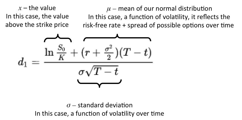
d1 represents the standardised distance between current stock price (S) and strike price (K) in terms of standard deviation, acounting the effect of time (T) and risk-free interest rate (r). It is used to calculate the probability that the option will be exercised (stock price exceeds the strike price at expiration).

d2 adjust d1 by sigma * sqrt(T), which represnts the volatility of the stock price over the option’s lifetime. d2 is used to calculate the present value of the paying the strike price at expiration, weighted by the probability.

Find the implied volatility using Newton-Raphson method

def implied_vol (S, K, T, r, price, max_iterations = 100, tol = 1.0e-5):
    sigma = 0.5
    for i in range(max_iterations):
        value = black_scholes_call_values(S, K, T, r, sigma)
        diff = value - price
        if abs(diff) < tol:
            break
        sigma = sigma + diff / (value - price)
    return sigma

Here I used the Newton-Raphson method to find the implied volatility. The method uses function’s derivative to iterately approximate the solution.

Newton-Raphson Formula: X_n+1 = X_n – f(X_n)/f'(X_n)

In the case of implied volatility calculation: The target is to solve for sigma such that the Black-Scholes formula equal the observed market price of the option. Define the function f(sigma) as the difference between the observed market price and the Black-Scholes.

The derivative f'(sigma) is the Vega of the option, which is: vega = S * sqrt(T) * N'(d1)

Thus, each iteration updates as: sigma(n+1) = sigma(n) – f(sigma(n)) / vega. Vega represent the rate of change of an option’s price with respect to changes in the implied volatility of the underlying asset. It qualifies how much the option price change for a 1% change in volatility.